Evaluation Climate Variability Modes CMIP6
CMIP6 Multi-Model Mean Context
Comparison with CMIP6 ensemble mean from 11 members.
Contributing models: ACCESS-ESM1-5, AWI-CM-1-1-MR, CNRM-CM6-1, CNRM-ESM2-1, EC-Earth3, FGOALS-g3, GISS-E2-1-G, INM-CM5-0, IPSL-CM6A-LR, MPI-ESM1-2-LR, MRI-ESM2-0
Synthesis
Related diagnostics
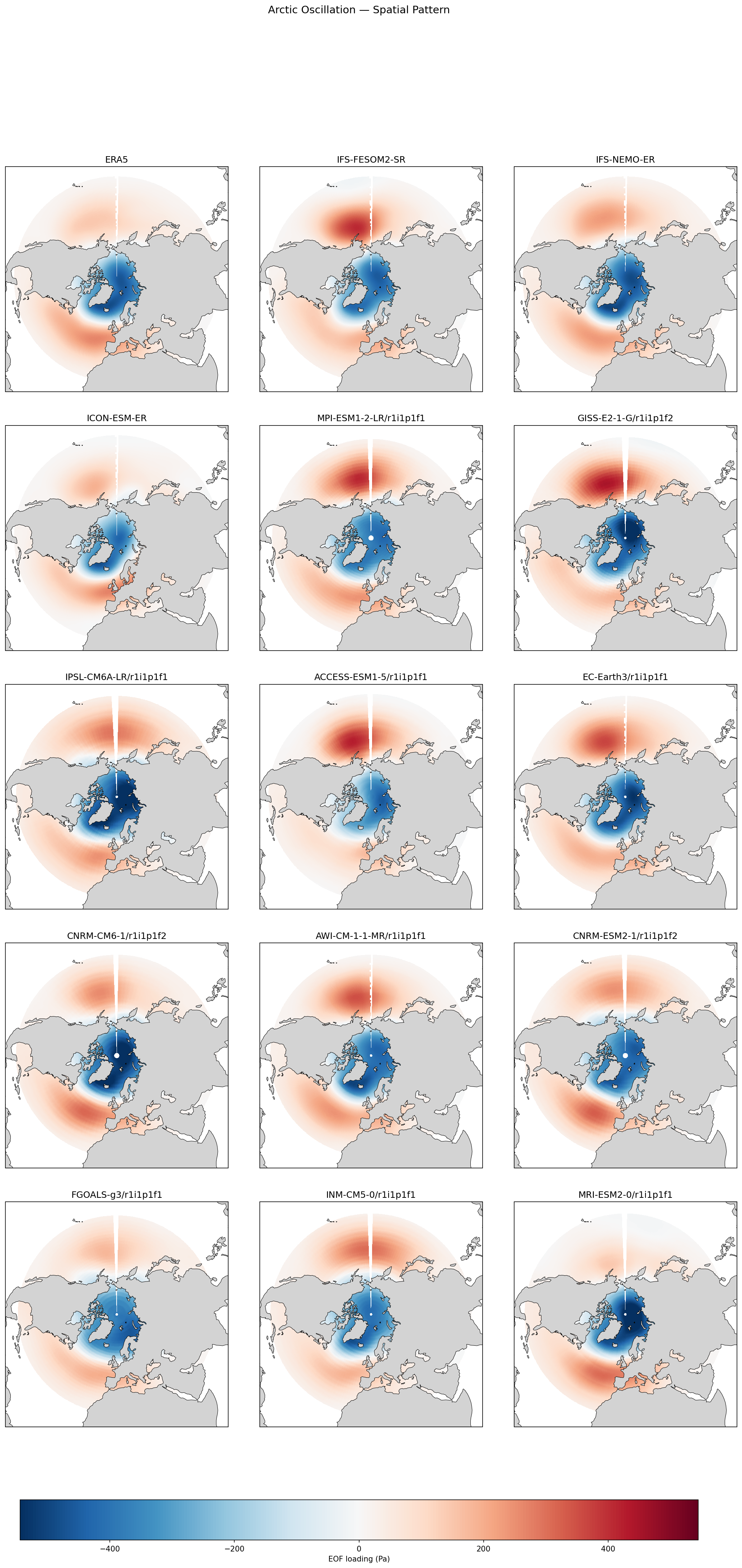
Arctic Oscillation — Spatial Pattern
| Variables | psl |
|---|---|
| Models | IFS-FESOM2-SR, IFS-NEMO-ER, ICON-ESM-ER |
| Reference Dataset | ERA5 |
| Units | Pa |
| Period | 1980–2014 |
| IFS-FESOM2-SR | Variance Explained: 0.21 |
| IFS-NEMO-ER | Variance Explained: 0.22 |
| ICON-ESM-ER | Variance Explained: 0.15 |
| ERA5 | Variance Explained: 0.20 |
Summary high
This diagnostic compares the spatial structure and explained variance of the Arctic Oscillation (AO) leading EOF pattern in sea level pressure across ERA5 reanalysis, three high-resolution EERIE models, and a suite of CMIP6 models.
Key Findings
- IFS-FESOM2-SR and IFS-NEMO-ER reproduce the ERA5 AO spatial pattern with high fidelity, capturing both the Arctic low and the mid-latitude high-pressure ring.
- The explained variance in the IFS models (20.9% for FESOM2-SR, 22.4% for NEMO-ER) closely matches ERA5 (19.9%), indicating a realistic representation of the mode's dominance.
- ICON-ESM-ER underestimates the explained variance (14.9%) and exhibits a noticeably weaker spatial loading pattern, particularly in the North Pacific sector.
- The high-resolution IFS models generally show sharper definition of the Atlantic and Pacific centers of action compared to several coarser CMIP6 models (e.g., INM-CM5-0, which is too weak).
Spatial Patterns
All models exhibit the classic annular structure with negative loading over the Arctic and positive loading over the mid-latitudes (Atlantic and Pacific). ERA5 shows two distinct positive centers in the North Atlantic and North Pacific. IFS-FESOM2-SR captures this duality exceptionally well. In contrast, ICON-ESM-ER shows a washed-out Pacific center. Some CMIP6 models (e.g., GISS-E2-1-G) show an overly intense or spatially extensive Pacific center.
Model Agreement
There is high agreement between the two IFS-based high-resolution models and ERA5. ICON-ESM-ER diverges by underestimating the mode's strength. The CMIP6 ensemble shows significant spread in pattern amplitude, placing the IFS models among the best performers relative to ERA5.
Physical Interpretation
The AO represents the primary mode of mass exchange between the Arctic and mid-latitudes, driven by internal atmospheric dynamics and guided by the storm tracks. The accurate variance explained and spatial structure in IFS simulations suggest a realistic representation of the Northern Hemisphere jet streams and storm track variability. The weaker pattern in ICON-ESM-ER implies either a less coherent annular mode or higher levels of noise/variability in other modes diluting the EOF1 signal.
Caveats
- Analysis is based on the first EOF only; higher-order modes (e.g., PNA) are not assessed here.
- The color scale saturates at ±500 Pa, potentially masking peak intensity differences in the strongest models (e.g., GISS-E2-1-G).
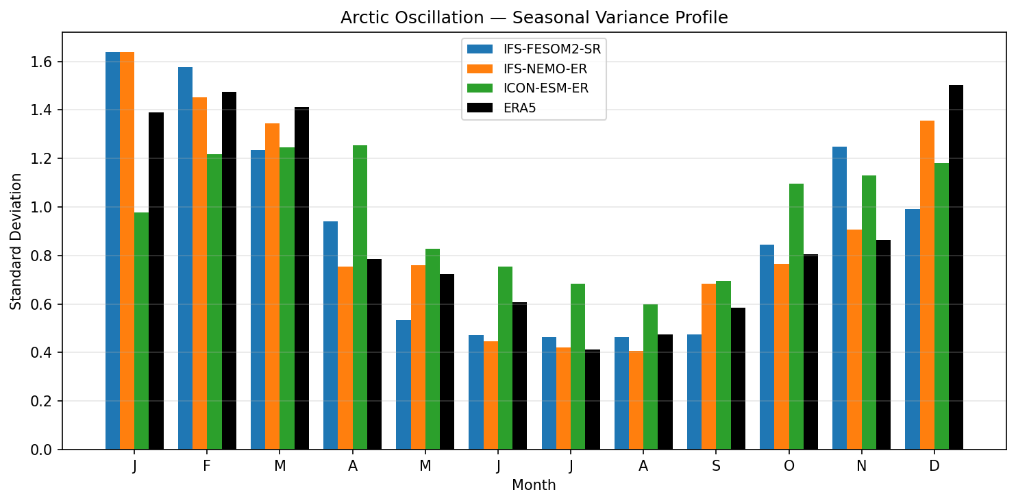
Arctic Oscillation — Seasonal Variance Profile
| Variables | psl |
|---|---|
| Models | IFS-FESOM2-SR, IFS-NEMO-ER, ICON-ESM-ER |
| Reference Dataset | ERA5 |
| Units | Pa |
| Period | 1980–2014 |
| IFS-FESOM2-SR | Peak Month: 1.00 · Peak Std: 1.64 · Annual Std: 1.00 |
| IFS-NEMO-ER | Peak Month: 1.00 · Peak Std: 1.64 · Annual Std: 1.00 |
| ICON-ESM-ER | Peak Month: 4.00 · Peak Std: 1.25 · Annual Std: 1.00 |
Summary high
This figure evaluates the seasonal cycle of Arctic Oscillation (AO) variability by comparing monthly standard deviations of the AO index in three high-resolution models against ERA5 reanalysis.
Key Findings
- ERA5 shows a pronounced seasonal cycle with variance peaking in winter (December-January, ~1.4–1.5) and reaching a minimum in summer (July, ~0.4).
- Both IFS-based models (IFS-FESOM2-SR and IFS-NEMO-ER) reproduce the observed phase accurately but overestimate the winter peak amplitude (January std dev ~1.64 vs ERA5 ~1.4).
- ICON-ESM-ER fails to capture the correct seasonality, exhibiting a delayed peak in April (~1.25) and systematically overestimating variability during the quiescent spring, summer, and autumn months.
Spatial Patterns
The observed AO exhibits strong seasonal locking, with standard deviations varying by a factor of 3-4 between winter active periods and summer quiescent periods.
Model Agreement
The two IFS models show high agreement with each other and good phase agreement with observations. ICON-ESM-ER diverges significantly, showing a distinct outlier behaviour in seasonality.
Physical Interpretation
The AO is dynamically most active in boreal winter due to vigorous tropospheric eddy activity and stratosphere-troposphere coupling. The IFS models capture this dynamical intensification well, though perhaps with excessive zonal flow variability in late winter. ICON's anomalous April peak and dampened winter variance suggest deficiencies in simulating the timing of the stratospheric vortex breakdown or the seasonal modulation of the Northern Hemisphere jet stream.
Caveats
- The AO is defined here by the leading EOF of sea level pressure; differences in the spatial loading pattern itself are not visible in this variance metric but could contribute to index differences.
- The analysis period (1980-2014) is sufficient but relatively short for robust statistics on decadal variability modulation of the AO.
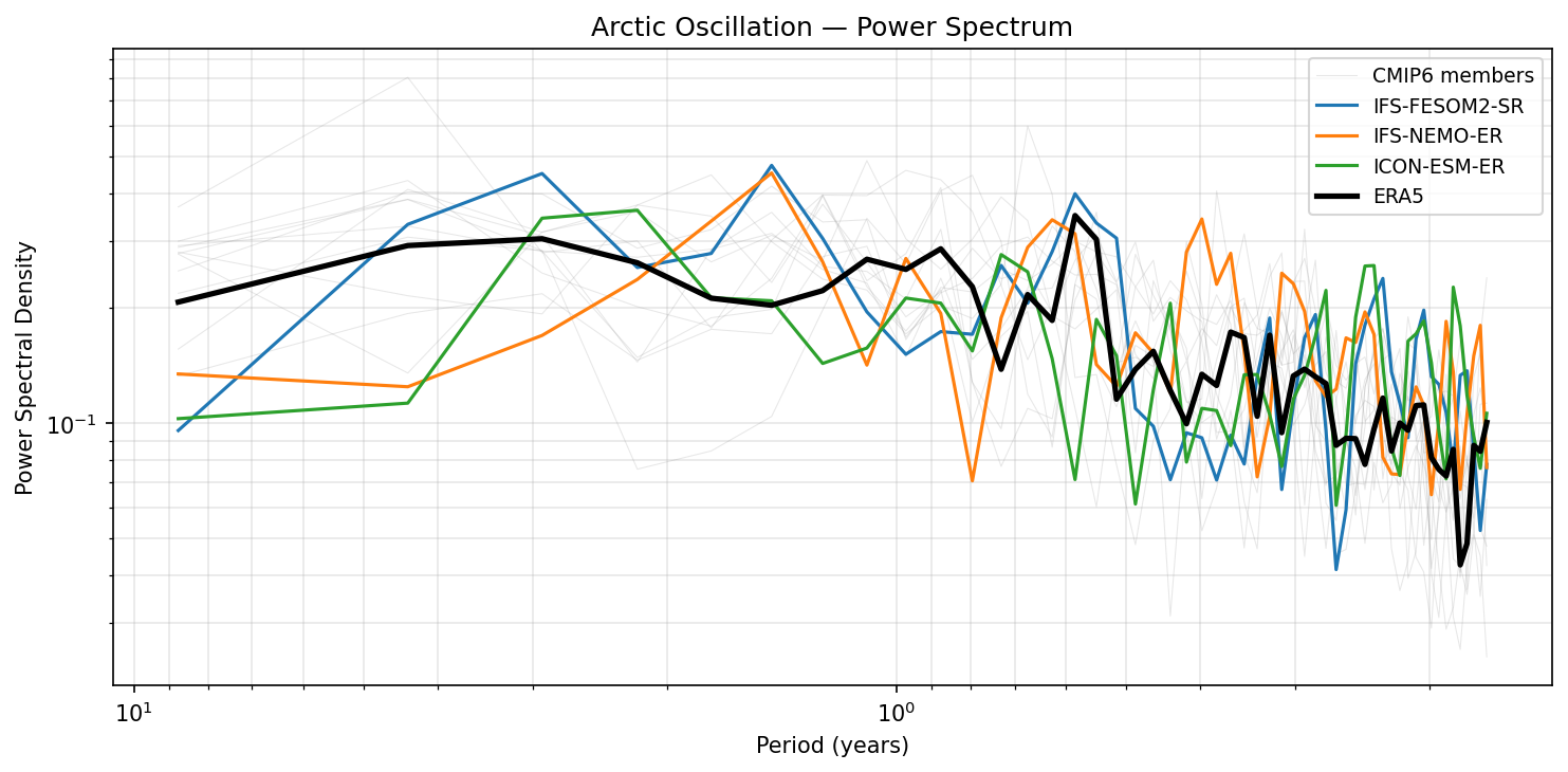
Arctic Oscillation — Power Spectrum
| Variables | psl |
|---|---|
| Models | IFS-FESOM2-SR, IFS-NEMO-ER, ICON-ESM-ER |
| Reference Dataset | ERA5 |
| Units | Pa |
| Period | 1980–2014 |
Summary high
This spectral analysis compares the variability of the Arctic Oscillation (AO) index in three high-resolution coupled models against ERA5 reanalysis and the CMIP6 ensemble over the 1980–2014 period. The models generally reproduce the observed spectral shape, but significant differences emerge in variability amplitude at interannual to decadal timescales.
Key Findings
- IFS-FESOM2-SR reproduces the decadal-scale (>5 years) power density of ERA5 remarkably well, whereas IFS-NEMO-ER and ICON-ESM-ER underestimate variability in this low-frequency band.
- In the interannual band (2–5 years), both IFS-based models (FESOM and NEMO) exhibit distinct spectral peaks that exceed the power found in ERA5, which shows a flatter plateau in this range.
- At sub-annual periods (<1 year), all three models closely track the ERA5 power spectrum and fall well within the CMIP6 ensemble spread, indicating a realistic representation of high-frequency atmospheric stochastic variability.
- ICON-ESM-ER consistently shows the lowest power spectral density across the interannual to decadal range, often tracking the lower bound of the CMIP6 ensemble spread.
Spatial Patterns
N/A (Temporal frequency analysis). The general pattern is a 'red' spectrum with power increasing at longer periods, consistent with theoretical expectations for the AO.
Model Agreement
Agreement is high at high frequencies (sub-annual) where all models converge with observations. Divergence increases significantly at low frequencies (>2 years), with IFS-FESOM2-SR aligning best with observations and ICON-ESM-ER showing the weakest low-frequency variability.
Physical Interpretation
The AO spectrum typically follows a red noise profile, resulting from the integration of stochastic atmospheric forcing. The divergence between IFS-FESOM2-SR and IFS-NEMO-ER (which share the same IFS atmospheric component) at low frequencies suggests that differences in ocean/sea-ice models or coupling strategies may influence the long-term persistence (memory) of the oscillation, although internal variability plays a strong role.
Caveats
- The analysis period (1980–2014) is relatively short (35 years), making the estimation of decadal spectral power statistically uncertain (few degrees of freedom).
- Differences between single model realizations at low frequencies may reflect internal variability rather than systematic physics biases, as indicated by the wide spread of the CMIP6 background ensemble.
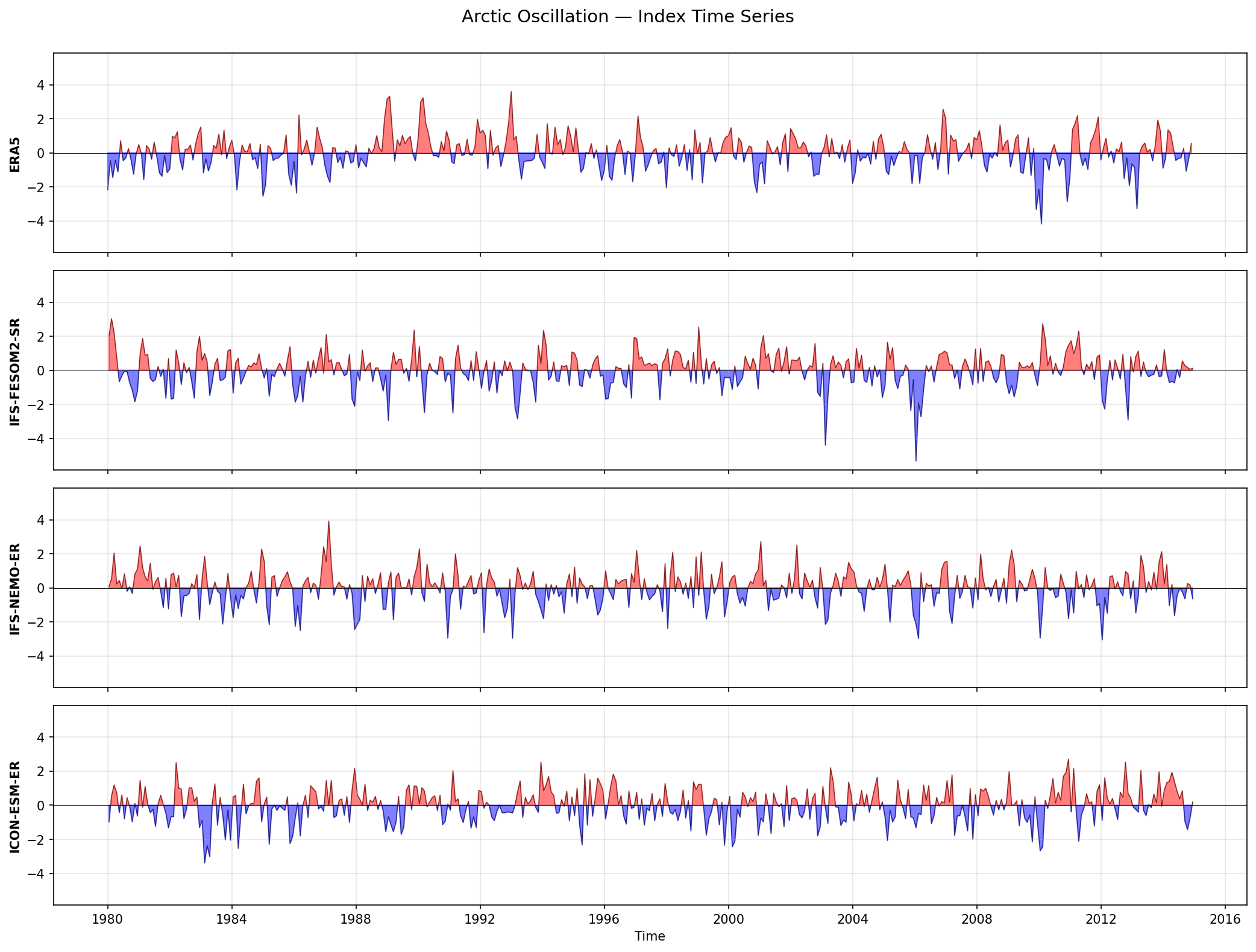
Arctic Oscillation — Index Time Series
| Variables | psl |
|---|---|
| Models | IFS-FESOM2-SR, IFS-NEMO-ER, ICON-ESM-ER |
| Reference Dataset | ERA5 |
| Units | Pa |
| Period | 1980–2014 |
| IFS-FESOM2-SR | Std: 1.00 · Mean: 0.00 |
| IFS-NEMO-ER | Std: 1.00 · Mean: 0.00 |
| ICON-ESM-ER | Std: 1.00 · Mean: 0.00 |
Summary high
This diagnostic figure compares standardized monthly Arctic Oscillation (AO) index time series from 1980–2014 for ERA5 reanalysis and three high-resolution coupled models (IFS-FESOM2-SR, IFS-NEMO-ER, ICON-ESM-ER), illustrating the models' ability to generate internal variability with realistic temporal characteristics.
Key Findings
- All three models reproduce the stochastic nature of the AO, exhibiting realistic vacillations between positive and negative phases without obvious periodic biases.
- The magnitude of variability is consistent with observations; models generate extreme events (index values exceeding ±3 to ±4 standard deviations) comparable to the major negative AO event seen in ERA5 around 2010.
- IFS-FESOM2-SR produces the most pronounced extreme negative excursion (approx. -5 sigma around simulated year 2006), demonstrating the capacity for strong blocking or stratospheric coupling events.
Spatial Patterns
As a time-series diagnostic, spatial patterns are not shown, but the temporal evolution in all panels is characterized by high-frequency (monthly) noise superimposed on interannual variability, with no discernible long-term trend over the 1980–2014 period.
Model Agreement
The models show high agreement with ERA5 in terms of statistical properties (amplitude distribution and event frequency). As these are free-running coupled simulations, the chronological timing of specific peaks and troughs does not match ERA5, which is the expected behavior.
Physical Interpretation
The realistic generation of AO variability suggests that the high-resolution models (approx. 10 km atmosphere) successfully resolve the eddy-mean flow interactions and Rossby wave breaking mechanisms that drive Northern Hemisphere annular mode variability. The presence of extreme negative events implies that the models likely capture disruptive dynamical processes such as sudden stratospheric warmings or high-latitude blocking.
Caveats
- The indices are standardized to unit variance (std=1.0), which masks potential biases in the absolute magnitude of Sea Level Pressure (SLP) variance or the spatial loading of the AO pattern.
- Without a power spectrum analysis, it is difficult to strictly quantify if the persistence (e-folding time) of the AO phases matches observations.
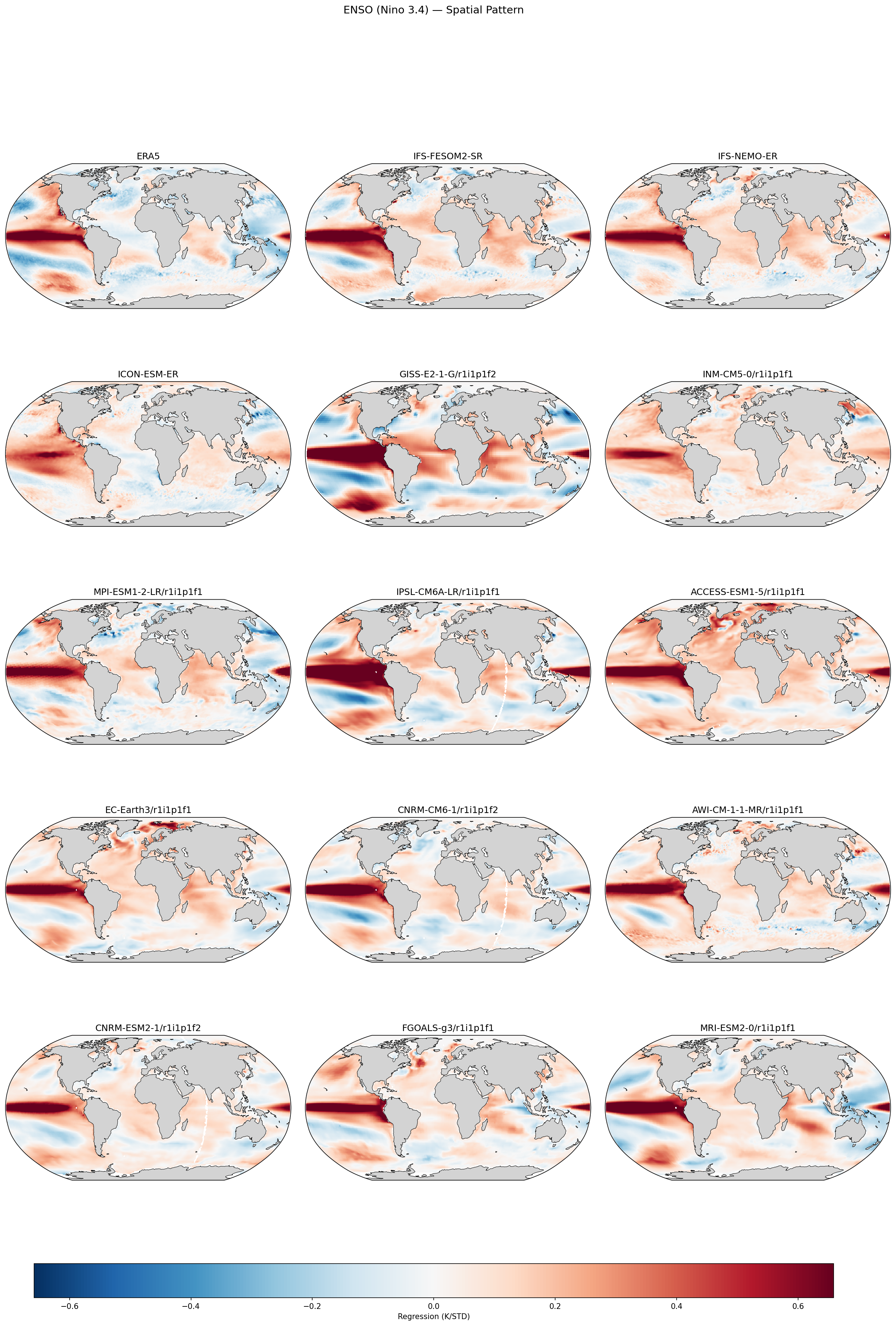
ENSO (Nino 3.4) — Spatial Pattern
| Variables | tos |
|---|---|
| Models | IFS-FESOM2-SR, IFS-NEMO-ER, ICON-ESM-ER, HadGEM3-GC5 |
| Reference Dataset | ESA_CCI |
| Units | K |
| Period | 1980–2014 |
Summary high
The diagnostic evaluates the spatial pattern of ENSO (SST regression onto Niño 3.4 index) in high-resolution EERIE models compared to ERA5 and a CMIP6 ensemble. The EERIE models generally reproduce the canonical tongue structure and meridional confinement well, though with variations in the longitudinal extent of the warming signal.
Key Findings
- IFS-FESOM2-SR and IFS-NEMO-ER exhibit robust ENSO spatial patterns with realistic meridional confinement of equatorial anomalies, outperforming lower-resolution CMIP6 outliers like GISS-E2-1-G which show excessive meridional spread.
- IFS-FESOM2-SR displays a westward bias in the extension of the equatorial warming tongue, with positive anomalies penetrating deeper into the western Pacific warm pool compared to ERA5 and IFS-NEMO-ER.
- IFS-NEMO-ER captures the transition to negative anomalies (the western Pacific horseshoe) more accurately than IFS-FESOM2-SR, aligning closely with the ERA5 reference.
- Global teleconnections, such as the Indian Ocean Basin Mode warming and the North Pacific PDO-like pattern, are well-captured by the high-resolution IFS models.
Spatial Patterns
The classic ENSO pattern—an elongated tongue of warming in the central/eastern equatorial Pacific flanked by a horseshoe of cooling in the west—is visible in the reference. EERIE models capture the basin-wide Indian Ocean warming response and the off-equatorial Pacific anomalies.
Model Agreement
There is high agreement between the high-resolution IFS models and the better-performing CMIP6 models (e.g., EC-Earth3, MRI-ESM2-0). However, the CMIP6 ensemble shows significant spread in pattern fidelity (e.g., GISS-E2-1-G is too broad; INM-CM5-0 is too weak), highlighting the value of the higher-resolution simulations.
Physical Interpretation
The spatial pattern reflects the Bjerknes feedback mechanism, where trade wind relaxation reinforces SST warming. The meridional confinement in high-resolution models suggests better resolved equatorial waveguide dynamics (Kelvin/Rossby waves). The westward shift in IFS-FESOM2-SR suggests a bias in the mean state cold tongue boundary or trade wind stress fetch.
Caveats
- The plot shows regression coefficients (K/STD), essentially normalizing the pattern amplitude; this does not show if the absolute variance of ENSO (amplitude in K) is correct.
- The reference is labelled ERA5 but metadata states ESA_CCI; since ERA5 assimilates SST, they are effectively consistent, but this distinction is noted.
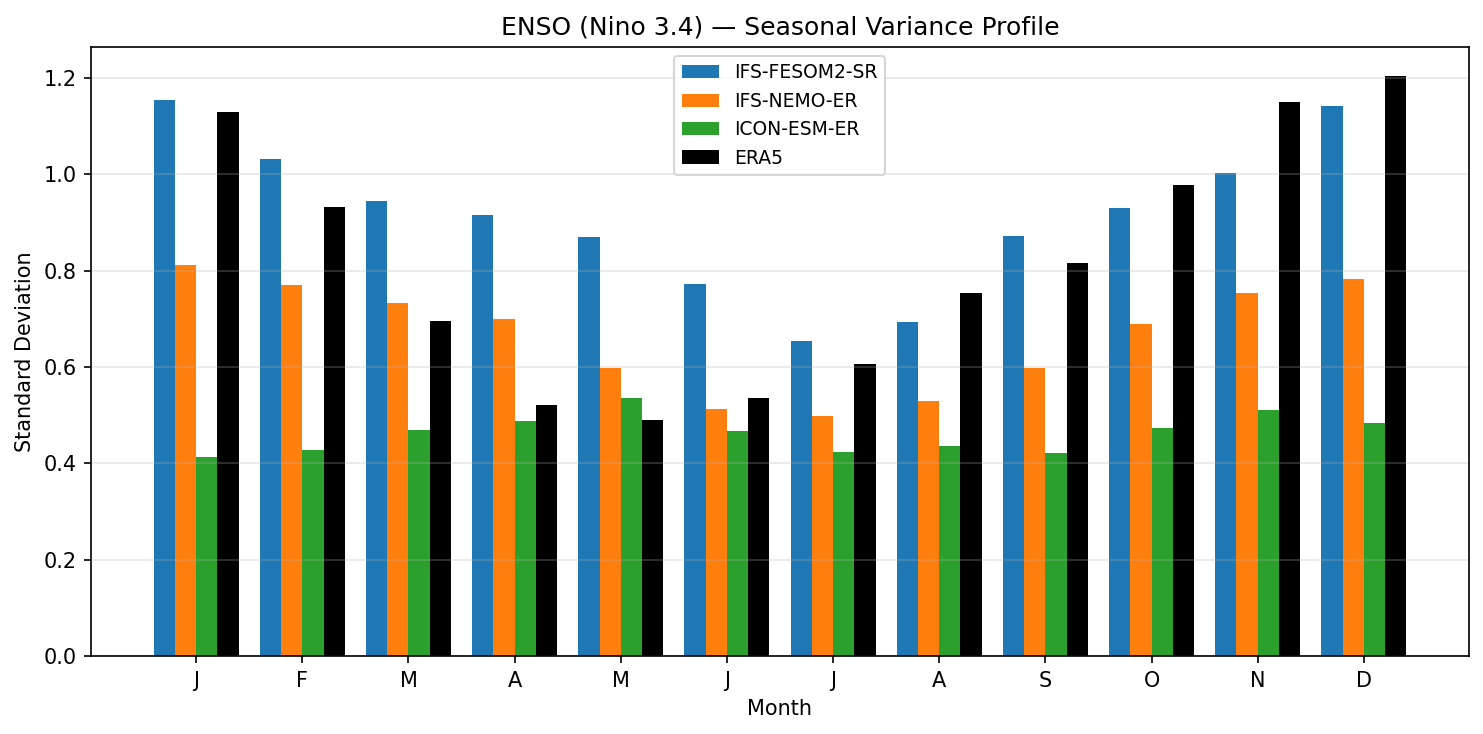
ENSO (Nino 3.4) — Seasonal Variance Profile
| Variables | tos |
|---|---|
| Models | IFS-FESOM2-SR, IFS-NEMO-ER, ICON-ESM-ER, HadGEM3-GC5 |
| Reference Dataset | ESA_CCI |
| Units | K |
| Period | 1980–2014 |
| IFS-FESOM2-SR | Peak Month: 1.00 · Peak Std: 1.15 · Annual Std: 0.93 |
| IFS-NEMO-ER | Peak Month: 1.00 · Peak Std: 0.81 · Annual Std: 0.67 |
| ICON-ESM-ER | Peak Month: 5.00 · Peak Std: 0.54 · Annual Std: 0.46 |
| HadGEM3-GC5 | Peak Month: 12.00 · Peak Std: 1.30 · Annual Std: 1.04 |
Summary high
This figure evaluates the seasonal phase locking of ENSO variability by comparing the monthly standard deviation of the Niño 3.4 SST index across four high-resolution models against ERA5.
Key Findings
- ERA5 displays the characteristic ENSO seasonal cycle, with variance peaking in boreal winter (DJF, ~1.2 K) and reaching a minimum in spring (AMJ, ~0.5 K).
- HadGEM3-GC5 captures the seasonal phasing well but overestimates variability, particularly in late autumn and early winter (peaking >1.3 K).
- IFS-FESOM2-SR reproduces the winter peak amplitude (~1.15 K) closely but fails to capture the spring minimum, maintaining excessive variability (>0.7 K) throughout the year.
- IFS-NEMO-ER underestimates ENSO variability year-round (peak ~0.8 K) but qualitatively captures the seasonal shape.
- ICON-ESM-ER exhibits critically weak variability (<0.55 K) with no discernible seasonal cycle, effectively failing to simulate ENSO dynamics.
Spatial Patterns
The analysis focuses on the temporal seasonal cycle (January-December). The observational 'spring predictability barrier' is evident as a variance minimum in ERA5 during April-June; this feature is only distinctly captured by HadGEM3-GC5 and weakly by IFS-NEMO-ER, whereas IFS-FESOM2-SR shows spuriously high variance during these months.
Model Agreement
There is substantial inter-model divergence in both amplitude and phase. HadGEM3-GC5 and IFS-FESOM2-SR are the most realistic in terms of winter magnitude, while IFS-NEMO-ER and ICON-ESM-ER are too damped. Only HadGEM3-GC5 successfully combines high amplitude with the correct seasonal phasing.
Physical Interpretation
The seasonal phase locking of ENSO arises from the seasonal modulation of the Bjerknes feedback and ocean-atmosphere coupling strength. The weak variability in ICON-ESM-ER and IFS-NEMO-ER suggests overly strong damping or insufficient coupling efficiency. Conversely, the high spring variance in IFS-FESOM2-SR suggests it does not capture the relaxation processes or stability usually present during the boreal spring.
Caveats
- The analysis uses ERA5 as the reference, which is generally consistent with observational SST products like HadISST or OISST for this metric.
- Standard deviation implies symmetric variability; it does not distinguish between El Niño and La Niña amplitude asymmetry.
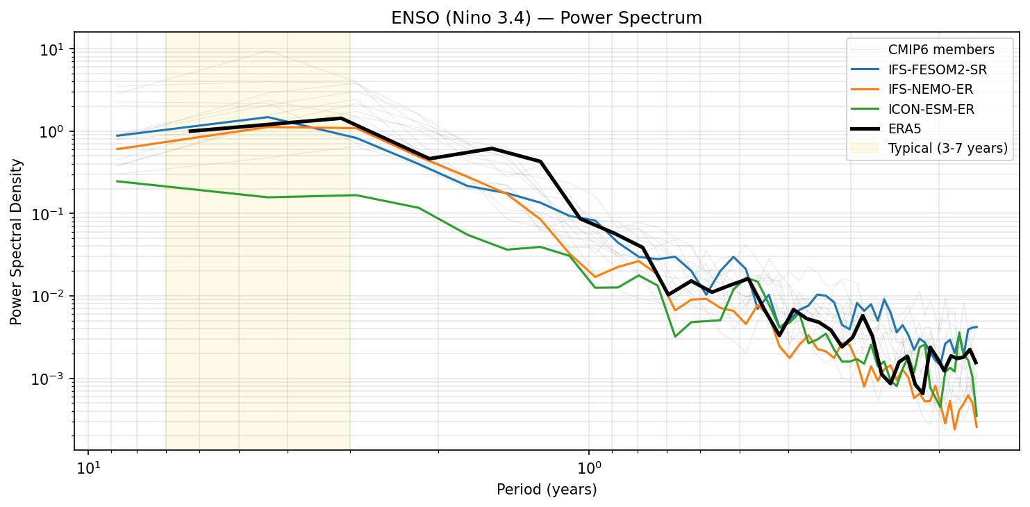
ENSO (Nino 3.4) — Power Spectrum
| Variables | tos |
|---|---|
| Models | IFS-FESOM2-SR, IFS-NEMO-ER, ICON-ESM-ER, HadGEM3-GC5 |
| Reference Dataset | ESA_CCI |
| Units | K |
| Period | 1980–2014 |
Summary high
This power spectrum analysis of the Niño 3.4 SST index evaluates the frequency and amplitude of ENSO variability in high-resolution models against ERA5 and CMIP6. HadGEM3-GC5 accurately reproduces the observed spectral peak, whereas ICON-ESM-ER exhibits severely suppressed variability.
Key Findings
- HadGEM3-GC5 shows the highest skill, closely matching the ERA5 power spectrum magnitude and shape within the typical 3-7 year ENSO band.
- ICON-ESM-ER is a distinct outlier with negligible ENSO variability; its power spectral density is roughly an order of magnitude lower than observations across all frequencies.
- Both IFS-based models (IFS-FESOM2-SR and IFS-NEMO-ER) capture the correct periodicity (peaking ~3-5 years) but slightly underestimate the amplitude of variability compared to ERA5.
- The CMIP6 ensemble (grey lines) shows a wide spread of ENSO amplitudes; ICON-ESM-ER falls well below the lower bound of this ensemble, while other EERIE models fall within the typical range.
Spatial Patterns
The analysis focuses on the temporal domain (periodicity). The critical observational feature is the broad spectral peak between 3 and 7 years (shaded yellow region), representing the irregular oscillation of El Niño/La Niña events.
Model Agreement
There is a strong divergence in model performance. HadGEM3-GC5 agrees well with ERA5. The two IFS models agree with each other (robustness across ocean components) but are slightly weaker than obs. ICON-ESM-ER disagrees significantly with both observations and the other models.
Physical Interpretation
The realistic spectrum in HadGEM3-GC5 suggests active and well-represented Bjerknes feedbacks (wind-thermocline-SST coupling). The suppression in ICON-ESM-ER indicates a failure in these coupling mechanisms, likely due to mean-state biases (e.g., a cold tongue error or excessive thermocline stability) that dampen the growth of SST anomalies.
Caveats
- The analysis period (1980–2014) is relatively short for resolving decadal variability, leading to noise at the low-frequency end (left side).
- Spectral analysis does not reveal phase synchronization or specific event reproduction, only the statistical characteristics of the variability.
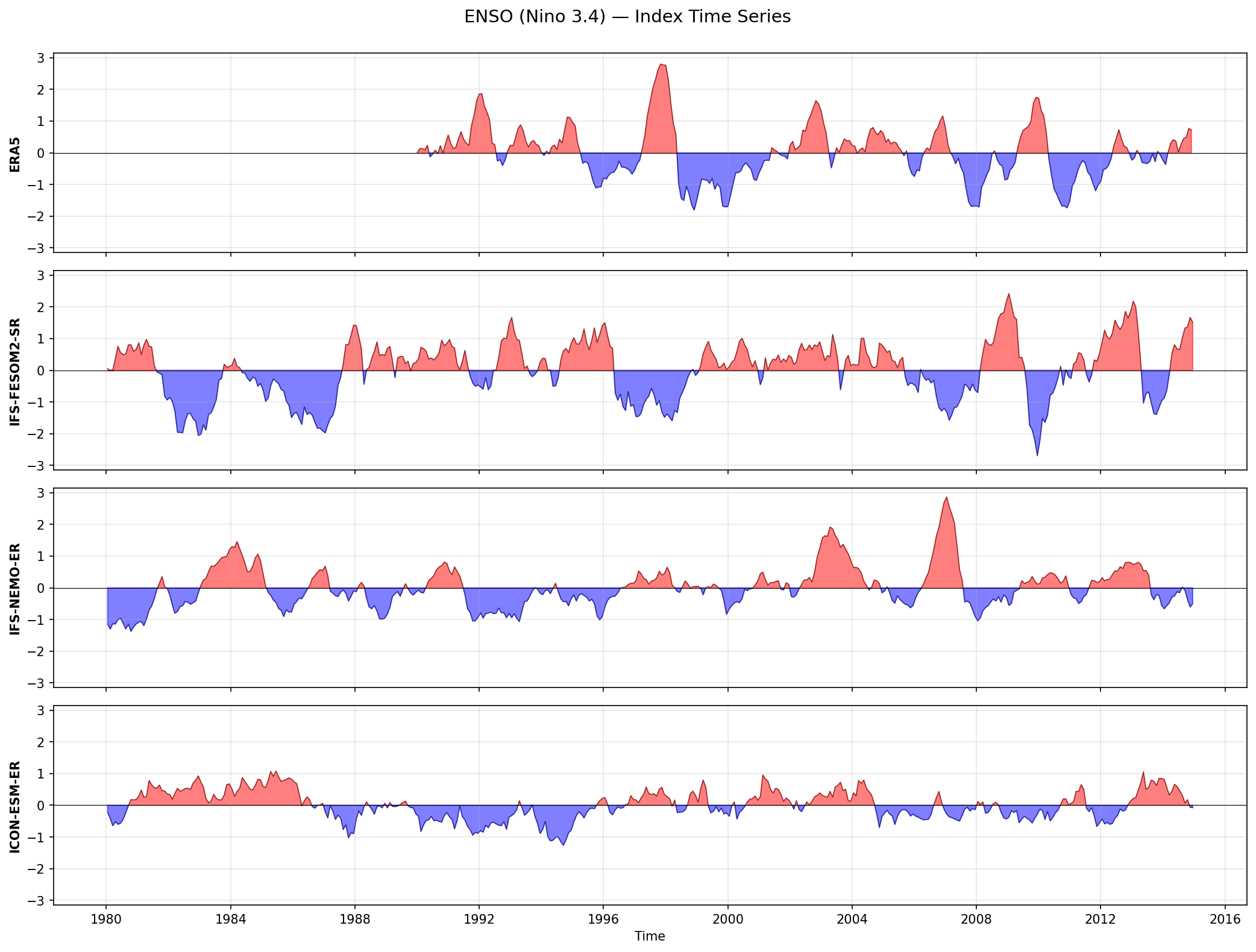
ENSO (Nino 3.4) — Index Time Series
| Variables | tos |
|---|---|
| Models | IFS-FESOM2-SR, IFS-NEMO-ER, ICON-ESM-ER, HadGEM3-GC5 |
| Reference Dataset | ESA_CCI |
| Units | K |
| Period | 1980–2014 |
| IFS-FESOM2-SR | Std: 0.93 · Mean: -0.00 |
| IFS-NEMO-ER | Std: 0.67 · Mean: 0.00 |
| ICON-ESM-ER | Std: 0.46 · Mean: 0.00 |
| HadGEM3-GC5 | Std: 1.04 · Mean: 0.00 |
Summary high
This figure compares the time evolution of the Niño 3.4 sea surface temperature anomaly index (ENSO) across four high-resolution coupled models and ERA5 observations for the period 1980–2014.
Key Findings
- IFS-FESOM2-SR demonstrates the most realistic ENSO simulation, with a standard deviation (0.93 K) close to observed values and a realistic irregular oscillation character.
- ICON-ESM-ER exhibits severely damped ENSO variability (std = 0.46 K), effectively lacking significant El Niño or La Niña events (anomalies rarely exceed ±1 K).
- HadGEM3-GC5 produces an overly energetic and regular ENSO cycle (std = 1.04 K), characterised by 'super-El Niño' events exceeding +3 K and a highly periodic, almost clock-like recurrence that lacks the chaotic nature of the real system.
- IFS-NEMO-ER underestimates ENSO amplitude (std = 0.67 K), producing variability that is too weak compared to observations.
Spatial Patterns
While this is a time series, the temporal 'pattern' of variability differs markedly: Observations and IFS-FESOM2-SR show chaotic, multi-scale intermittency (typical 3-7 year band). HadGEM3-GC5 shows a distinct, quasi-periodic 'sawtooth' pattern with sharp, high-amplitude warm events. ICON-ESM-ER shows only low-amplitude, higher-frequency fluctuations.
Model Agreement
There is substantial divergence in model performance regarding ENSO amplitude and frequency. IFS-FESOM2-SR is the only model that closely matches the statistical properties of the observational record, while others drift to either damped (ICON, IFS-NEMO) or hyper-active (HadGEM3) extremes.
Physical Interpretation
The diversity suggests different balances in the Bjerknes feedback loop (wind-SST coupling). ICON-ESM-ER and IFS-NEMO-ER likely suffer from weak coupling or excessive damping (thermal or momentum) in the equatorial Pacific. Conversely, HadGEM3-GC5 appears to have an overly strong positive feedback or insufficient damping, leading to a 'perfect oscillator' regime common in some high-bias models.
Caveats
- The ERA5 observational time series appears to be missing or zero-filled prior to approximately 1989 in this plot, limiting visual comparison for the first decade.
- As these are free-running coupled simulations, the timing (phase) of ENSO events is not expected to match historical observations; evaluation is based solely on statistical properties (amplitude, frequency, regularity).
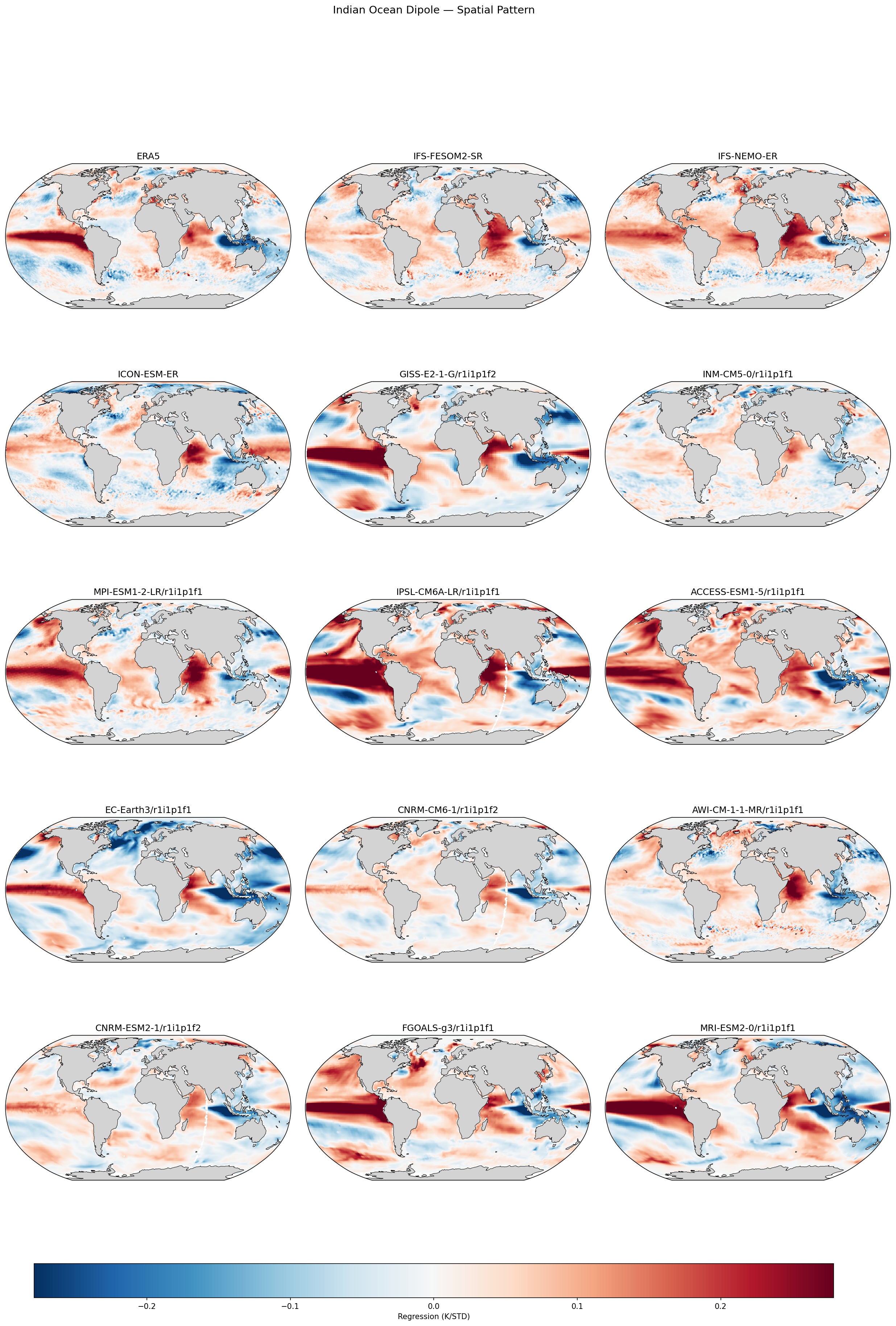
Indian Ocean Dipole — Spatial Pattern
| Variables | tos |
|---|---|
| Models | IFS-FESOM2-SR, IFS-NEMO-ER, ICON-ESM-ER, HadGEM3-GC5 |
| Reference Dataset | ESA_CCI |
| Units | K |
| Period | 1980–2014 |
Summary high
The diagnostic evaluates the spatial structure of the Indian Ocean Dipole (IOD) in high-resolution EERIE models against ERA5 and a CMIP6 ensemble. The EERIE models generally capture the characteristic zonal SST gradient (eastern cooling, western warming) well, with some exhibiting strong coupling to Pacific ENSO variability.
Key Findings
- IFS-FESOM2-SR and IFS-NEMO-ER show excellent structural agreement with ERA5 in the Indian Ocean, correctly placing the eastern cooling center off Sumatra.
- HadGEM3-GC5 exhibits a very high-amplitude pattern with intense eastern cooling and a dominant El Niño-like teleconnection in the Pacific, suggesting strong ENSO-IOD coupling.
- ICON-ESM-ER reproduces the dipole but with a slightly less spatially coherent eastern pole compared to the IFS and HadGEM3 configurations.
- Several CMIP6 models (e.g., GISS-E2-1-G, INM-CM5-0) struggle to resolve the sharp eastern pole, whereas the high-resolution EERIE models generally resolve this feature well, likely due to better representation of coastal upwelling dynamics.
Spatial Patterns
The dominant pattern is a zonal dipole in the tropical Indian Ocean: negative SST anomalies (cooling) in the southeast near Sumatra/Java and positive anomalies (warming) in the west. A positive correlation tongue extends into the central/eastern Pacific, reflecting the known association between positive IOD events and El Niño.
Model Agreement
EERIE models show high consistency in the Indian Ocean basin, often outperforming lower-resolution CMIP6 outliers. Disagreement is highest in the magnitude of the Pacific teleconnection, with HadGEM3-GC5 and some CMIP6 models (IPSL-CM6A-LR, MRI-ESM2-0) showing much stronger Pacific signals than ERA5 or IFS-FESOM2-SR.
Physical Interpretation
The patterns are driven by the Bjerknes feedback: easterly wind anomalies lift the thermocline in the eastern Indian Ocean (cooling) and depress it in the west (warming). The Pacific signal illustrates the 'atmospheric bridge' where ENSO modifies the Walker circulation to trigger or amplify IOD events. Models with intense Pacific patterns may have excessive ENSO variance or overly rigid inter-basin coupling.
Caveats
- The figures show simple regression, not partial regression; thus, the Pacific signal represents the combined IOD-ENSO mode rather than pure IOD variability.
- Color saturation in HadGEM3-GC5 suggests amplitudes may be overestimated relative to ERA5.
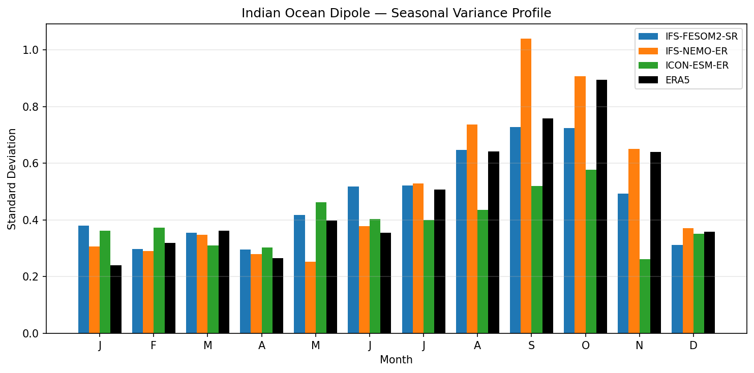
Indian Ocean Dipole — Seasonal Variance Profile
| Variables | tos |
|---|---|
| Models | IFS-FESOM2-SR, IFS-NEMO-ER, ICON-ESM-ER, HadGEM3-GC5 |
| Reference Dataset | ESA_CCI |
| Units | K |
| Period | 1980–2014 |
| IFS-FESOM2-SR | Peak Month: 9.00 · Peak Std: 0.73 · Annual Std: 0.50 |
| IFS-NEMO-ER | Peak Month: 9.00 · Peak Std: 1.04 · Annual Std: 0.57 |
| ICON-ESM-ER | Peak Month: 10.00 · Peak Std: 0.58 · Annual Std: 0.41 |
| HadGEM3-GC5 | Peak Month: 9.00 · Peak Std: 1.13 · Annual Std: 0.70 |
Summary high
This figure evaluates the seasonal cycle of Indian Ocean Dipole (IOD) variability, revealing significant inter-model spread in amplitude despite generally correct phase-locking for most models.
Key Findings
- ERA5 observations show a distinct variance peak in October (~0.9 K), reflecting the characteristic autumn phase-locking of the IOD.
- HadGEM3-GC5 significantly overestimates variability, peaking at >1.1 K in September and maintaining excessive variance through December.
- ICON-ESM-ER fails to capture the seasonal amplification, producing a flat variance profile (~0.4–0.5 K) that severely underestimates the autumn peak.
- IFS-NEMO-ER and IFS-FESOM2-SR capture the seasonal cycle shape reasonably well, though IFS-NEMO overestimates the September peak while IFS-FESOM tends to underestimate variability in late autumn (Oct-Dec).
Spatial Patterns
The observational baseline exhibits a classic IOD lifecycle: low variance in boreal spring (Feb-Apr), growth during summer, peak in autumn (Sept-Oct), and decay in winter. HadGEM3-GC5 shows a delayed decay with anomalously high variance persisting into winter. ICON-ESM-ER lacks distinct seasonality entirely.
Model Agreement
Models disagree substantially on the magnitude of IOD variability, ranging from <0.6 K (ICON) to >1.1 K (HadGEM3). While IFS and HadGEM3 agree on the timing of the onset (growing from June), they tend to peak in September, one month earlier than the ERA5 October peak.
Physical Interpretation
The IOD is driven by Bjerknes feedbacks (wind-thermocline-SST coupling) in the tropical Indian Ocean. The weak variability in ICON-ESM-ER likely points to mean-state biases, such as a too-deep thermocline in the eastern pole or weak zonal winds, which suppress these feedbacks. Conversely, the excessive variability in HadGEM3-GC5 suggests overly strong coupling or a mean state that is too unstable. The early peak in models (Sept vs Oct) is a common bias in coupled systems, often related to errors in the seasonal march of the ITCZ.
Caveats
- The legend identifies the observation as ERA5, while metadata lists ESA_CCI; for SST-based indices, these are generally consistent but distinct products.
- The analysis period (1980–2014) captures limited IOD events, making variance statistics sensitive to individual extreme years.
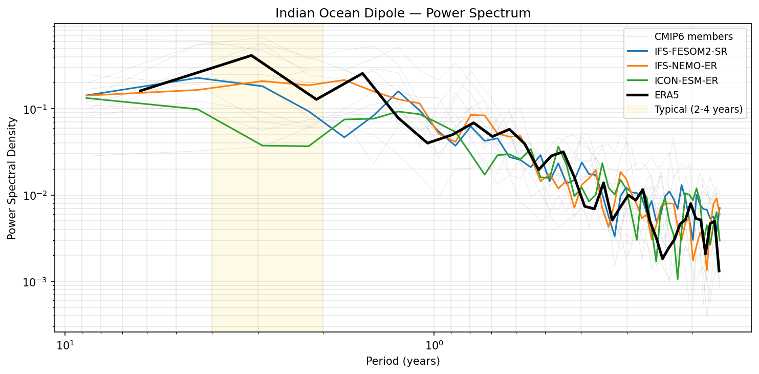
Indian Ocean Dipole — Power Spectrum
| Variables | tos |
|---|---|
| Models | IFS-FESOM2-SR, IFS-NEMO-ER, ICON-ESM-ER, HadGEM3-GC5 |
| Reference Dataset | ESA_CCI |
| Units | K |
| Period | 1980–2014 |
Summary high
This figure displays the power spectral density of the Indian Ocean Dipole (IOD) index for four high-resolution climate models compared to ERA5 reanalysis and the CMIP6 ensemble.
Key Findings
- HadGEM3-GC5 significantly overestimates IOD variability, showing excessive power spectral density across interannual timescales (>2 years) well above ERA5 and the CMIP6 range.
- ICON-ESM-ER underestimates variability in the typical 2-4 year IOD band, with power levels falling near the bottom of the CMIP6 ensemble spread.
- IFS-FESOM2-SR and IFS-NEMO-ER show reasonable agreement with observations, capturing the spectral shape and magnitude better than the other high-res models, though they slightly underestimate the peak power relative to ERA5.
- ERA5 observations show a distinct spectral peak in the 2.5–4 year band, which is broadly reproduced in period by HadGEM3 (though exaggerated in amplitude) but washed out in ICON.
Spatial Patterns
The observed spectrum features a primary peak of variability at periods of 3–4 years. HadGEM3-GC5 exhibits a broad, high-amplitude maximum in this same frequency band extending to decadal scales. In contrast, ICON-ESM-ER displays a relatively flat spectrum lacking a distinct interannual peak.
Model Agreement
There is substantial divergence among the high-resolution models. They bracket the observations, with HadGEM3-GC5 being too energetic and ICON-ESM-ER being too damped. The IFS models (both NEMO and FESOM variants) cluster in the middle, offering the best match to the observational reference.
Physical Interpretation
The excessive power in HadGEM3-GC5 suggests overly strong Bjerknes feedback or insufficient thermal damping in the tropical Indian Ocean, leading to high-amplitude dipole events. Conversely, the suppressed variability in ICON-ESM-ER implies weak ocean-atmosphere coupling or excessive damping of SST anomalies. The IFS models strike a better balance in coupled dynamics.
Caveats
- The analysis period (1980–2014) is relatively short for robustly estimating power spectral density at decadal timescales (left side of the plot).
- Internal variability can significantly influence spectral peaks in short records, as indicated by the wide spread of individual CMIP6 members.
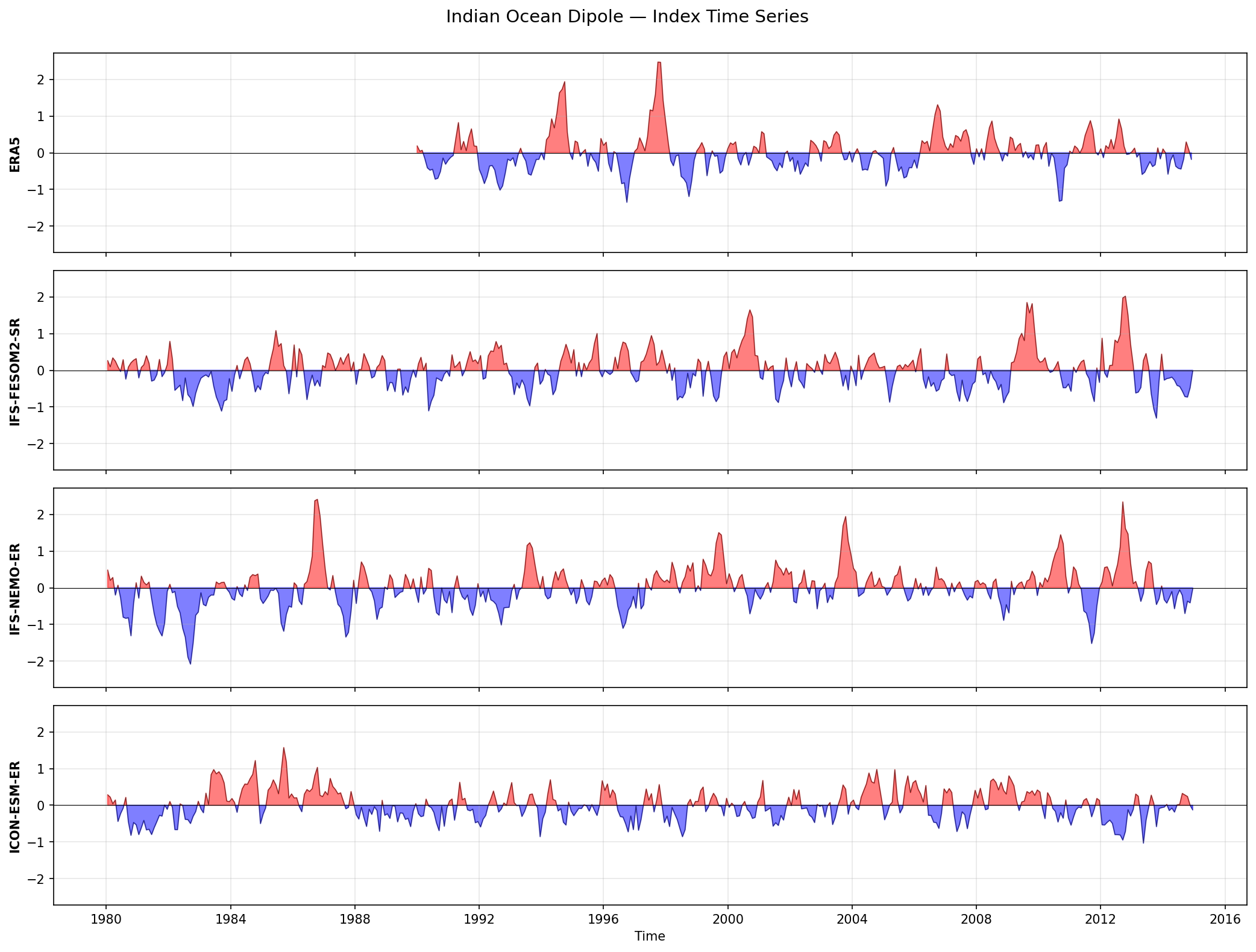
Indian Ocean Dipole — Index Time Series
| Variables | tos |
|---|---|
| Models | IFS-FESOM2-SR, IFS-NEMO-ER, ICON-ESM-ER, HadGEM3-GC5 |
| Reference Dataset | ESA_CCI |
| Units | K |
| Period | 1980–2014 |
| IFS-FESOM2-SR | Std: 0.50 · Mean: 0.00 |
| IFS-NEMO-ER | Std: 0.57 · Mean: 0.00 |
| ICON-ESM-ER | Std: 0.41 · Mean: -0.00 |
| HadGEM3-GC5 | Std: 0.70 · Mean: 0.00 |
Summary high
This figure displays the time series of the Indian Ocean Dipole (IOD) index from 1980 to 2014 for four high-resolution coupled climate models compared to ERA5 reanalysis.
Key Findings
- There is a significant spread in IOD variability amplitude across the models, ranging from suppressed to hyper-active.
- HadGEM3-GC5 exhibits the strongest variability (STD ~0.70 K), with frequent extreme positive and negative events exceeding 2 K magnitude, likely overestimating observed variance.
- ICON-ESM-ER shows the weakest variability (STD ~0.41 K), failing to produce extreme IOD events comparable to the strong events seen in the observational record (e.g., 1997, 2006).
- IFS-FESOM2-SR and IFS-NEMO-ER produce intermediate variability (STD ~0.50 K and ~0.57 K respectively), with peak magnitudes that align reasonably well with the active phases of the observed record.
Spatial Patterns
The time series show the characteristic irregular interannual oscillation of the IOD. All models capture the quasi-periodic nature of the phenomenon (typically 2-5 years), though the frequency and persistence of events vary.
Model Agreement
Models diverge considerably in amplitude. HadGEM3-GC5 is the most energetic, while ICON-ESM-ER is the most damped. The two IFS-based models (FESOM2 and NEMO) cluster in the middle, suggesting that the ocean model formulation (unstructured vs. structured grid) has a moderate impact on IOD magnitude within the same atmospheric framework.
Physical Interpretation
The IOD relies on Bjerknes feedback mechanisms involving wind-SST-thermocline interactions in the equatorial Indian Ocean. The high variance in HadGEM3-GC5 suggests overly strong coupling or a thermocline that is too sensitive to wind forcing (possibly too shallow). Conversely, ICON-ESM-ER's damped response suggests weak coupling or biases in the mean state (e.g., thermocline depth or zonal SST gradient) that inhibit the growth of anomalies.
Caveats
- The ERA5 observational reference (top panel) appears to be missing data (flat line at zero) prior to ~1989, limiting the validation period to the latter half of the time series.
- As these are free-running coupled simulations, the phase and timing of individual events are not expected to match observations; evaluation is based on statistical properties (amplitude, frequency) only.
North Atlantic Oscillation — Spatial Pattern
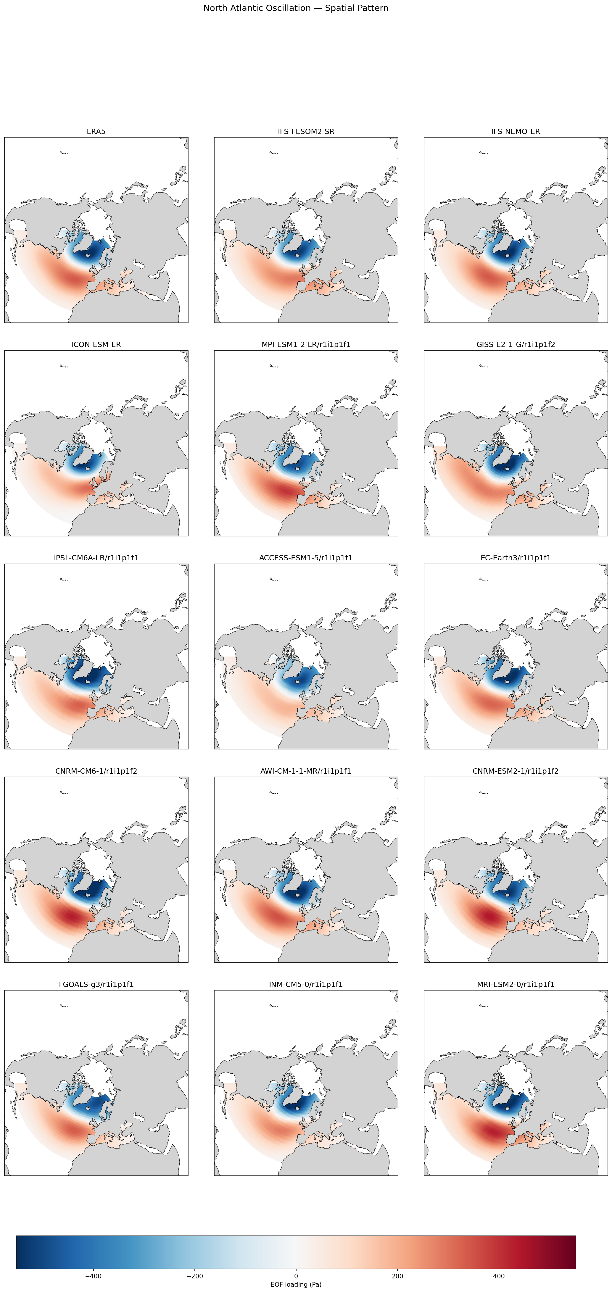
| Variables | psl |
|---|---|
| Models | IFS-FESOM2-SR, IFS-NEMO-ER, ICON-ESM-ER |
| Reference Dataset | ERA5 |
| Units | Pa |
| Period | 1980–2014 |
| IFS-FESOM2-SR | Variance Explained: 0.33 |
| IFS-NEMO-ER | Variance Explained: 0.35 |
| ICON-ESM-ER | Variance Explained: 0.27 |
| ERA5 | Variance Explained: 0.35 |
Summary high
This figure compares the spatial pattern (EOF1 of sea level pressure) and variance explained of the North Atlantic Oscillation (NAO) across ERA5 reanalysis, three high-resolution EERIE models, and a selection of CMIP6 models.
Key Findings
- IFS-NEMO-ER reproduces the ERA5 NAO pattern with remarkable fidelity, capturing both the spatial structure and the fraction of variance explained (35.3% vs 34.7% in ERA5).
- IFS-FESOM2-SR also performs well (32.8% variance explained), though the positive southern node (Azores High) is slightly less intense than in IFS-NEMO-ER.
- ICON-ESM-ER significantly underestimates the strength of the NAO mode, showing paler EOF loadings and explaining only 27.1% of the total variance, placing it at the lower end of performance compared to the IFS models.
- The spread within the CMIP6 ensemble is large, ranging from weak patterns (INM-CM5-0) to very strong dipoles (CNRM-ESM2-1), providing context that the IFS models are performing at or above the level of the best standard-resolution models.
Spatial Patterns
The classic dipole structure features a low-pressure anomaly over Iceland/Greenland and a high-pressure anomaly extending from the Azores across the Atlantic. IFS-NEMO-ER and ERA5 show a robust, well-defined southern node extending into Europe. ICON-ESM-ER and some CMIP6 models (e.g., ACCESS-ESM1-5, INM-CM5-0) exhibit a washed-out southern lobe, indicating a weaker meridional pressure gradient anomaly.
Model Agreement
There is high agreement between ERA5 and the two IFS-based models (NEMO and FESOM2). ICON-ESM-ER diverges by showing a weaker signal. The IFS models generally outperform the median CMIP6 representation, aligning closely with high-performing CMIP6 models like EC-Earth3.
Physical Interpretation
The NAO reflects the internal variability of the North Atlantic eddy-driven jet stream. The strong performance of IFS-NEMO-ER suggests it correctly resolves the storm track dynamics and the exchange of atmospheric mass between the subtropical high and subpolar low. The reduced variance in ICON-ESM-ER implies the model may have a less persistent or weaker jet stream variability, or that the variability is partitioned differently across EOF modes.
Caveats
- The analysis is restricted to the first EOF; if a model's NAO is split between modes (degenerate), this diagnostic might underrepresent it.
- Units are in Pascals; visual comparison of intensity relies on color saturation, which clearly shows ICON is weaker.
North Atlantic Oscillation — Seasonal Variance Profile
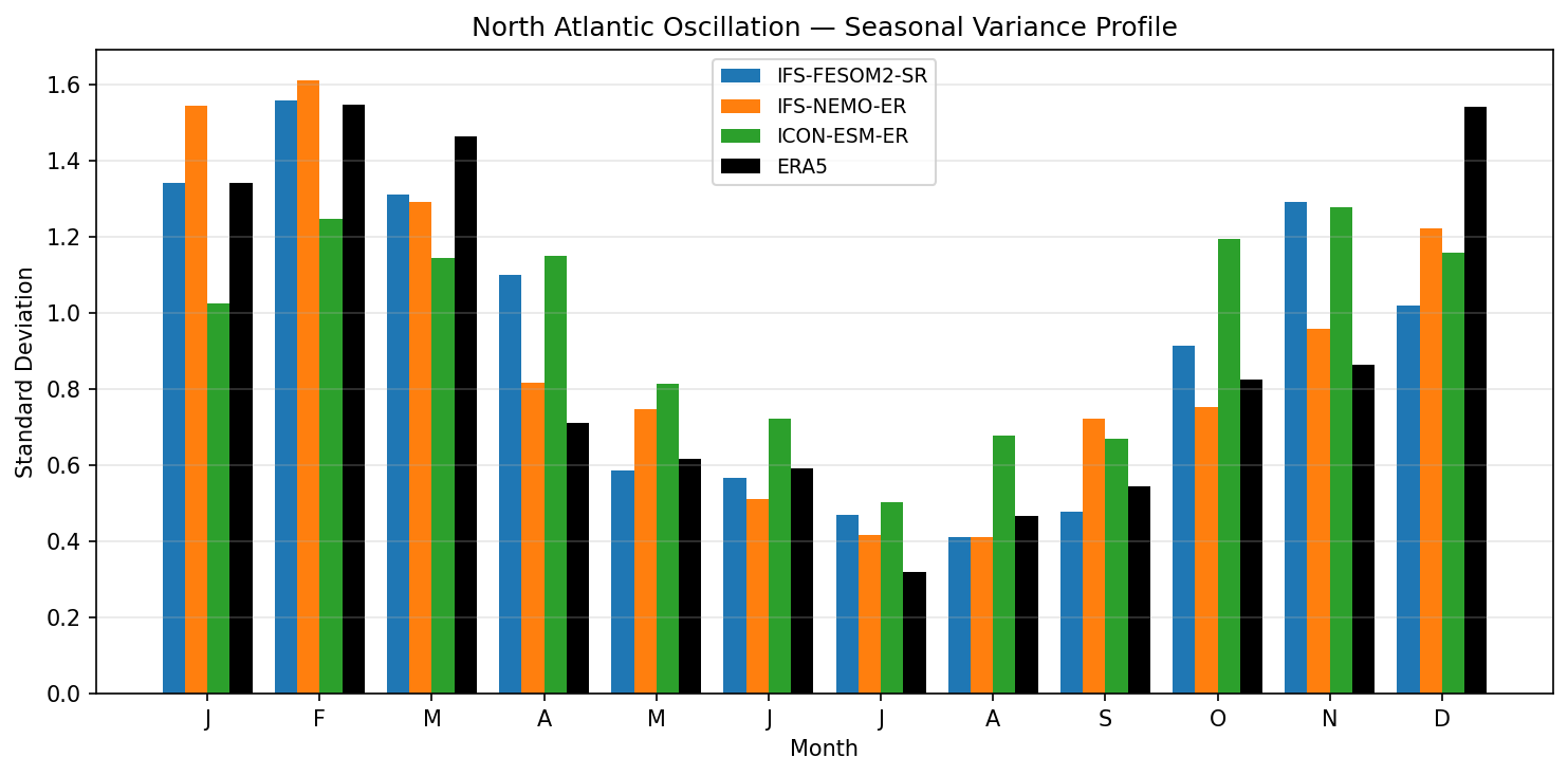
| Variables | psl |
|---|---|
| Models | IFS-FESOM2-SR, IFS-NEMO-ER, ICON-ESM-ER |
| Reference Dataset | ERA5 |
| Units | Pa |
| Period | 1980–2014 |
| IFS-FESOM2-SR | Peak Month: 2.00 · Peak Std: 1.56 · Annual Std: 1.00 |
| IFS-NEMO-ER | Peak Month: 2.00 · Peak Std: 1.61 · Annual Std: 1.00 |
| ICON-ESM-ER | Peak Month: 11.00 · Peak Std: 1.28 · Annual Std: 1.00 |
Summary high
This figure evaluates the seasonal cycle of North Atlantic Oscillation (NAO) variability by plotting the monthly standard deviation of the index for three models against ERA5 reanalysis.
Key Findings
- All models significantly underestimate NAO variability in December compared to ERA5, suggesting a delayed onset of peak winter variability.
- IFS-FESOM2-SR shows excellent agreement with ERA5 in late winter (Jan-Feb) and the summer minimum, but shares the December low bias.
- ICON-ESM-ER exhibits a flattened seasonal cycle, systematically underestimating winter variability (DJF) and overestimating variability in transition seasons (especially August–November).
- IFS-NEMO-ER generally captures the winter peak magnitude but tends to overestimate variability in January and February compared to ERA5.
Spatial Patterns
The observed (ERA5) NAO variability follows a strong seasonal cycle, peaking in winter (Dec-Feb standard deviation > 1.3) and reaching a minimum in summer (Jul standard deviation < 0.4).
Model Agreement
IFS-based models (FESOM and NEMO) agree well with the observed seasonal structure (strong winter/weak summer), whereas ICON-ESM-ER diverges significantly with a muted seasonal amplitude. All models agree on the underestimation of December variability.
Physical Interpretation
The NAO reflects the variability of the eddy-driven jet stream. The high winter variance corresponds to vigorous storm track activity. ICON-ESM-ER's flattened cycle suggests it fails to sufficiently modulate storm track stability between seasons, maintaining excessive wave activity in autumn and insufficient variance in winter. The delayed winter peak (weak December) across all models implies a systematic lag in establishing the fully developed winter circulation regime.
Caveats
- The indices are likely normalized over the full annual cycle (annual_std ~ 1.0), meaning values reflect relative seasonal redistribution of variance.
- Only one realization per model is shown, so internal variability could influence single-month peaks.
North Atlantic Oscillation — Power Spectrum
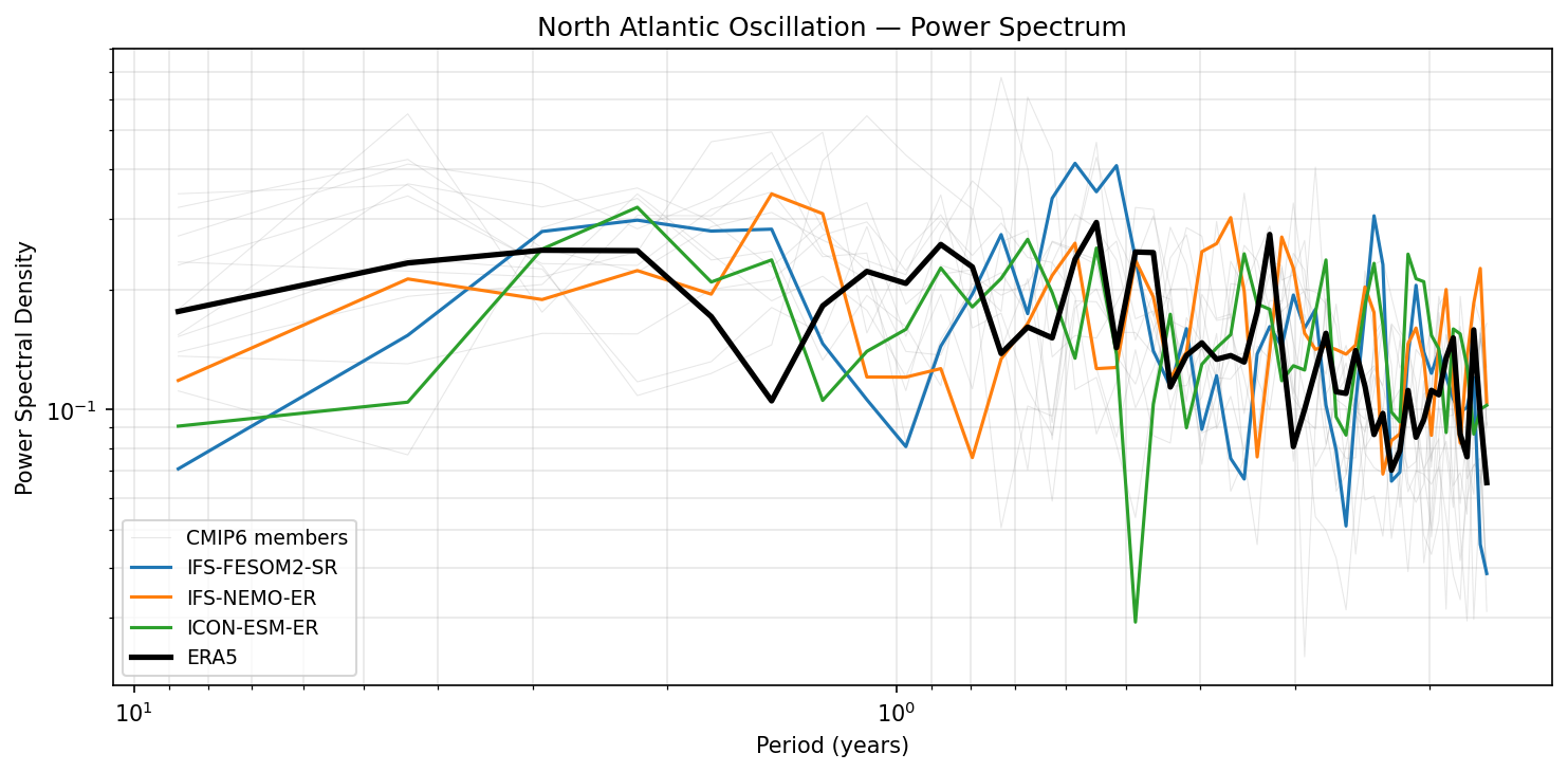
| Variables | psl |
|---|---|
| Models | IFS-FESOM2-SR, IFS-NEMO-ER, ICON-ESM-ER |
| Reference Dataset | ERA5 |
| Units | Pa |
| Period | 1980–2014 |
Summary medium
This power spectrum analysis of the North Atlantic Oscillation (NAO) compares three high-resolution models against ERA5 and the CMIP6 ensemble over the 1980–2014 period. The models generally reproduce the characteristic broadband, quasi-red noise spectrum of the NAO, though they tend to underestimate variability at decadal timescales.
Key Findings
- ERA5 displays a relatively flat spectral density across interannual timescales (2–10 years), consistent with the stochastic nature of the NAO.
- IFS-FESOM2-SR and ICON-ESM-ER underestimate power density at the longest periods (>8 years) relative to ERA5, indicating weaker decadal variability.
- IFS-NEMO-ER shows the closest agreement with ERA5 in the 2–8 year band, while ICON-ESM-ER exhibits a distinct drop in power at sub-annual periods (~0.4 years).
- All high-resolution models fall generally within the spread of the CMIP6 ensemble (grey lines), avoiding spurious dominant periodicities.
Spatial Patterns
N/A (Frequency domain analysis). The spectra show highest power at low frequencies (decadal) decreasing towards high frequencies (sub-annual), typical of 'red' geophysical noise.
Model Agreement
Models agree on the broad spectral shape (no single dominant peak). Divergence is highest at decadal scales (left side), where IFS-NEMO-ER aligns best with ERA5, while ICON-ESM-ER and IFS-FESOM2-SR are less energetic.
Physical Interpretation
The NAO is primarily driven by internal atmospheric dynamics (Rossby wave breaking), resulting in a largely white or slightly red spectrum. The models' success in capturing the broadband nature implies reasonable representation of these chaotic dynamics. The deficiency in low-frequency power in some models might suggest insufficient coupling with slow oceanic modes (e.g., AMV) or stratospheric variability that typically enhances decadal persistence.
Caveats
- The analysis period (1980–2014) is short (35 years), making spectral estimates at decadal periods (>10 years) statistically uncertain due to small sample size.
- Sub-annual features (right side) may be influenced by how monthly anomalies were constructed or temporal aliasing.
North Atlantic Oscillation — Index Time Series
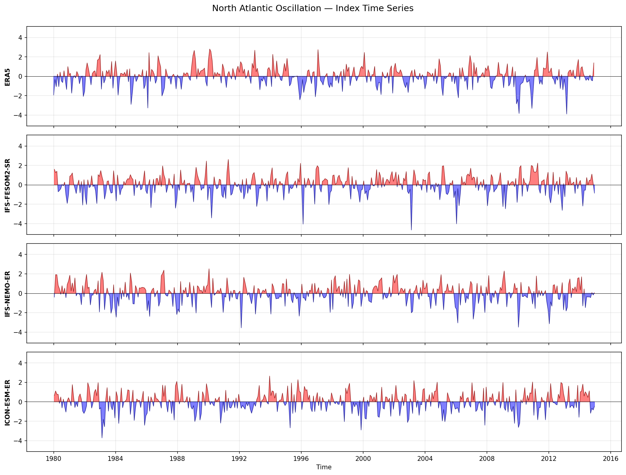
| Variables | psl |
|---|---|
| Models | IFS-FESOM2-SR, IFS-NEMO-ER, ICON-ESM-ER |
| Reference Dataset | ERA5 |
| Units | Pa |
| Period | 1980–2014 |
| IFS-FESOM2-SR | Std: 1.00 · Mean: -0.00 |
| IFS-NEMO-ER | Std: 1.00 · Mean: 0.00 |
| ICON-ESM-ER | Std: 1.00 · Mean: 0.00 |
Summary high
This figure displays the time evolution of the North Atlantic Oscillation (NAO) index from 1980 to 2014 for ERA5 reanalysis and three high-resolution coupled models. As expected for free-running simulations, the models do not reproduce the specific timing of historical events but demonstrate realistic amplitude, frequency, and statistical variability of the NAO mode.
Key Findings
- All three models (IFS-FESOM2-SR, IFS-NEMO-ER, ICON-ESM-ER) exhibit realistic variability, with index magnitudes generally fluctuating between ±3 standard deviations, consistent with the dynamic range seen in ERA5.
- The temporal character of the variability (frequency of phase reversals) in the models is visually comparable to observations, indicating they capture the characteristic stochastic timescales of North Atlantic atmospheric variability without excessive persistence.
- IFS-FESOM2-SR simulates a particularly strong negative excursion (below -4 SD around year 2003), demonstrating the model's capability to generate extreme blocking conditions comparable to the historic 2009/2010 event observed in ERA5.
Spatial Patterns
While the specific timing of phase changes varies due to internal variability, the models reproduce the 'red' noise characteristic of the NAO. ERA5 shows the known historical positive phase dominance in the early 1990s and the extreme negative dip in 2010; model realizations show similar stochastic excursions but at random intervals.
Model Agreement
There is high agreement across models regarding the statistical properties (variance, range, fluctuation frequency) of the NAO. Phases are uncorrelated with ERA5 and each other, which is the correct behavior for free-running coupled simulations.
Physical Interpretation
The realistic index behavior implies that the models' high-resolution atmospheric components (~10 km) correctly resolve the meridional pressure gradient fluctuations between the Icelandic Low and Azores High. The ability to generate index values beyond ±3 SD suggests that non-linear dynamical processes, such as Rossby wave breaking and atmospheric blocking, are active and realistic.
Caveats
- Since the indices are standardized (std ≈ 1), this figure assesses temporal statistics only and does not reveal if the spatial loading patterns (magnitude of pressure anomalies in Pa) are correct.
- Direct year-to-year comparison is not applicable as these are not assimilated runs.
Pacific Decadal Oscillation — Spatial Pattern
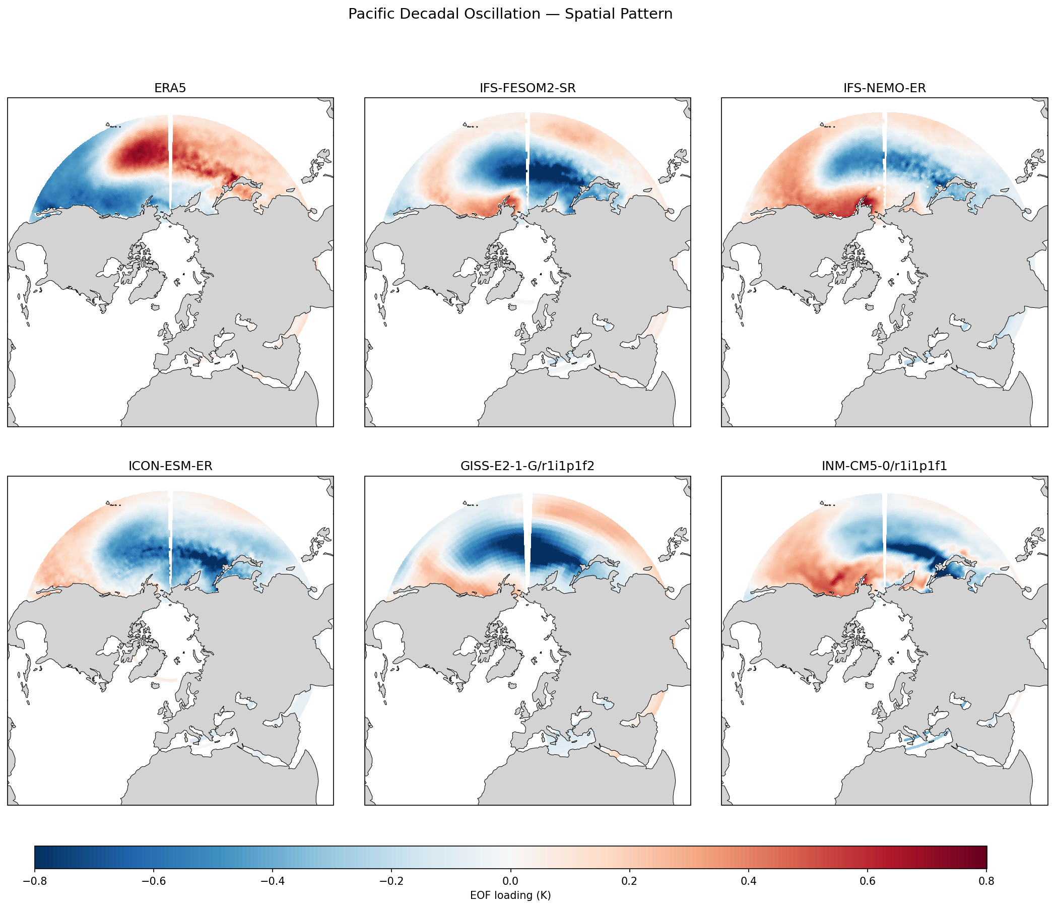
| Variables | tos |
|---|---|
| Models | IFS-FESOM2-SR, IFS-NEMO-ER, ICON-ESM-ER, HadGEM3-GC5 |
| Reference Dataset | ESA_CCI |
| Units | K |
| Period | 1980–2014 |
| IFS-FESOM2-SR | Variance Explained: 0.14 |
| IFS-NEMO-ER | Variance Explained: 0.12 |
| ICON-ESM-ER | Variance Explained: 0.13 |
| HadGEM3-GC5 | Variance Explained: 0.14 |
| ERA5 | Variance Explained: 0.19 |
Summary high
The EERIE models (IFS-FESOM2-SR, IFS-NEMO-ER, ICON-ESM-ER, HadGEM3-GC5) successfully reproduce the canonical horseshoe spatial pattern of the Pacific Decadal Oscillation (PDO), capturing the dipole between the central North Pacific and the North American coast.
Key Findings
- All high-resolution models exhibit the correct spatial structure of the PDO, characterized by anomalies of one sign in the central North Pacific (Kuroshio-Oyashio Extension region) and the opposite sign along the west coast of North America.
- The ERA5 reference plot displays the negative phase of the PDO (warm central, cold coastal) while all models display the positive phase (cold central, warm coastal); taking this arbitrary EOF sign convention into account, spatial agreement is excellent.
- Models consistently underestimate the fraction of variance explained by the PDO (12-14%) compared to ERA5 (~19%), suggesting that the PDO mode is less dominant relative to total variability in the simulations than in observations.
- HadGEM3-GC5 and IFS-FESOM2-SR show particularly sharp gradients in the Kuroshio-Oyashio Extension region, likely benefiting from higher ocean resolution compared to the smoother patterns seen in the lower-resolution CMIP6 models (e.g., GISS-E2-1-G).
Spatial Patterns
The dominant feature is the zonal elongation of SST anomalies along the Kuroshio-Oyashio Extension (approx. 40°N) and the horseshoe-shaped anomaly of opposite sign wrapping along the North American coast and into the subtropics. The high-resolution models resolve the narrow frontal nature of the western Pacific anomaly better than the coarser CMIP6 examples.
Model Agreement
There is strong inter-model agreement on the spatial footprint of the PDO. Quantitatively, HadGEM3-GC5 explains the most variance (14.2%) among models, closest to ERA5, while IFS-NEMO-ER explains the least (12.1%).
Physical Interpretation
The PDO pattern results from the ocean's integration of atmospheric noise (Aleutian Low variability) and Rossby wave dynamics affecting the Kuroshio-Oyashio Extension. The realistic representation of the western boundary current separation in these eddy-rich/eddy-permitting models likely contributes to the well-defined central Pacific anomalies.
Caveats
- The sign of the first EOF is arbitrary; the ERA5 panel shows the opposite sign (negative phase) relative to the models (positive phase), requiring mental inversion for comparison.
- Grid artifacts (white lines) are visible in the IFS-NEMO and IFS-FESOM plots, corresponding to mesh singularities or domain boundaries.
Pacific Decadal Oscillation — Seasonal Variance Profile
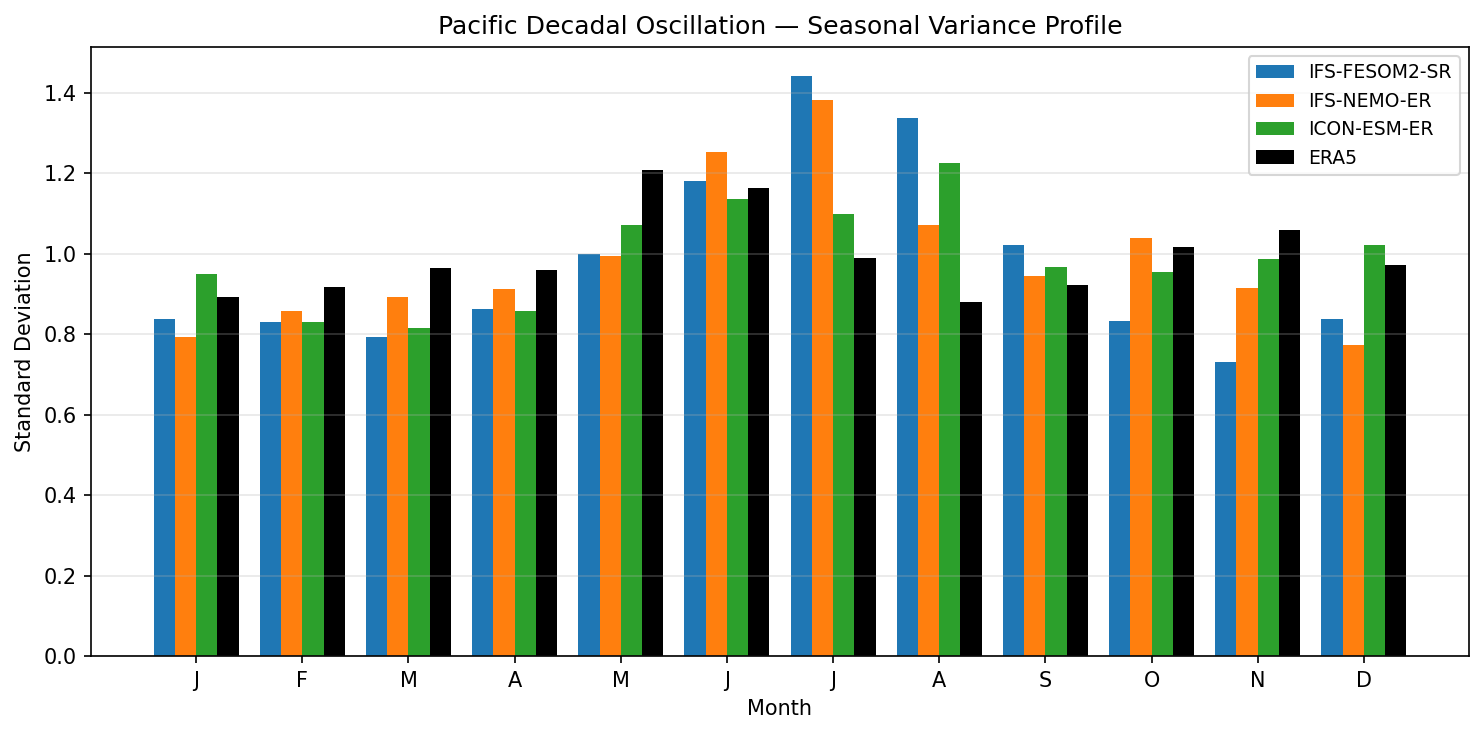
| Variables | tos |
|---|---|
| Models | IFS-FESOM2-SR, IFS-NEMO-ER, ICON-ESM-ER, HadGEM3-GC5 |
| Reference Dataset | ESA_CCI |
| Units | K |
| Period | 1980–2014 |
| IFS-FESOM2-SR | Peak Month: 7.00 · Peak Std: 1.44 · Annual Std: 1.00 |
| IFS-NEMO-ER | Peak Month: 7.00 · Peak Std: 1.38 · Annual Std: 1.00 |
| ICON-ESM-ER | Peak Month: 8.00 · Peak Std: 1.22 · Annual Std: 1.00 |
| HadGEM3-GC5 | Peak Month: 8.00 · Peak Std: 1.19 · Annual Std: 1.00 |
Summary high
All four high-resolution models exhibit a systematic bias in the seasonality of Pacific Decadal Oscillation (PDO) variability, peaking in late summer (July–August) rather than the observed late-spring (May–June) maximum.
Key Findings
- There is a systematic phase delay in peak PDO variance: ERA5 shows maximum variability in May–June (~1.2), while all models peak later in July (IFS models) or August (ICON, HadGEM3).
- IFS-FESOM2-SR and IFS-NEMO-ER significantly overestimate the magnitude of summer variability, with July standard deviations exceeding 1.4 compared to observational values of ~1.0.
- HadGEM3-GC5 and ICON-ESM-ER capture the magnitude of the variance peak better than the IFS models but still exhibit the late-summer timing bias.
- Winter (DJF) variance, which is critical for PDO-related teleconnections, is generally well-simulated across all models, oscillating around the observational standard deviation of ~0.9–1.0.
Spatial Patterns
The analysis focuses on the temporal seasonal cycle rather than spatial maps. The dominant pattern is a shifted seasonal cycle of variance: observations show a Spring/early-Summer maximum, while models show a distinct mid-to-late Summer maximum.
Model Agreement
The two IFS-based models (coupled to FESOM2 and NEMO) show high agreement with each other, suggesting the atmospheric component (IFS) or coupling strategy drives the excessive summer variance. ICON and HadGEM3 form a second cluster with lower summer variance but similar phase errors. All models agree on the delay relative to ERA5.
Physical Interpretation
The PDO is driven by the integration of atmospheric stochastic forcing, with SST variance generally inversely proportional to mixed layer depth (MLD). The model peak in July/August aligns with the annual minimum in MLD, suggesting the models may be exhibiting a simple mixed-layer response to forcing. The observed peak in May/June implies that in reality, other factors (e.g., seasonal changes in atmospheric forcing strength, damping, or reemergence dynamics) modulate this relationship, which the models fail to capture. The excessive summer variance in IFS runs could indicate too-shallow summer MLDs or insufficient surface heat flux damping.
Caveats
- Since the indices are standardized (annual standard deviation = 1.0), this figure assesses the relative distribution of variance across the seasonal cycle, not the absolute magnitude of SST anomalies.
- The discrepancy between the legend (ERA5) and metadata (ESA_CCI) for observations is minor, as both reanalysis and satellite products are consistent for low-frequency SST modes like the PDO.
Pacific Decadal Oscillation — Power Spectrum
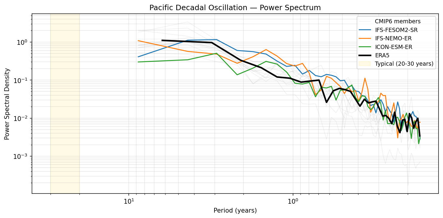
| Variables | tos |
|---|---|
| Models | IFS-FESOM2-SR, IFS-NEMO-ER, ICON-ESM-ER, HadGEM3-GC5 |
| Reference Dataset | ESA_CCI |
| Units | K |
| Period | 1980–2014 |
Summary medium
The power spectrum of the Pacific Decadal Oscillation (PDO) index for the period 1980–2014 shows that the evaluated high-resolution models generally reproduce the observed red-noise spectral characteristics, though systematic differences in variance amplitude exist at interannual timescales.
Key Findings
- All models successfully capture the general 'red noise' spectral slope (power increasing with period) characteristic of the PDO.
- ICON-ESM-ER systematically underestimates variability at periods longer than 2 years compared to ERA5 and the other high-resolution models.
- IFS-NEMO-ER and IFS-FESOM2-SR exhibit slightly higher power than ERA5 in the 5–10 year band, likely reflecting strong ENSO teleconnections projecting onto the PDO mode.
- HadGEM3-GC5 shows the closest agreement with the ERA5 spectral density across the resolved 1–15 year range.
Spatial Patterns
While this is a temporal diagnostic, the spectral distribution highlights that variability is concentrated at low frequencies. The 'typical' 20–30 year PDO peak falls outside the reliably resolved range of the 35-year analysis period.
Model Agreement
Inter-model agreement is relatively good for high-frequency variability (<2 years). Divergence increases at lower frequencies, with ICON-ESM-ER acting as a low-variance outlier and IFS variants tending towards higher variance than ERA5.
Physical Interpretation
The spectra reflect the integration of stochastic atmospheric forcing (Aleutian Low) and ENSO variability (peak visible ~5-7 years) by the North Pacific ocean mixed layer. The lower power in ICON-ESM-ER suggests either weak atmospheric forcing or insufficient oceanic persistence (thermal inertia) in the North Pacific.
Caveats
- The 1980–2014 analysis period (35 years) is too short to statistically resolve the canonical 20–30 year PDO timescale indicated by the shaded region.
- The low-frequency end of the spectrum is subject to high uncertainty due to the limited number of realizations/cycles in the record.
Pacific Decadal Oscillation — Index Time Series
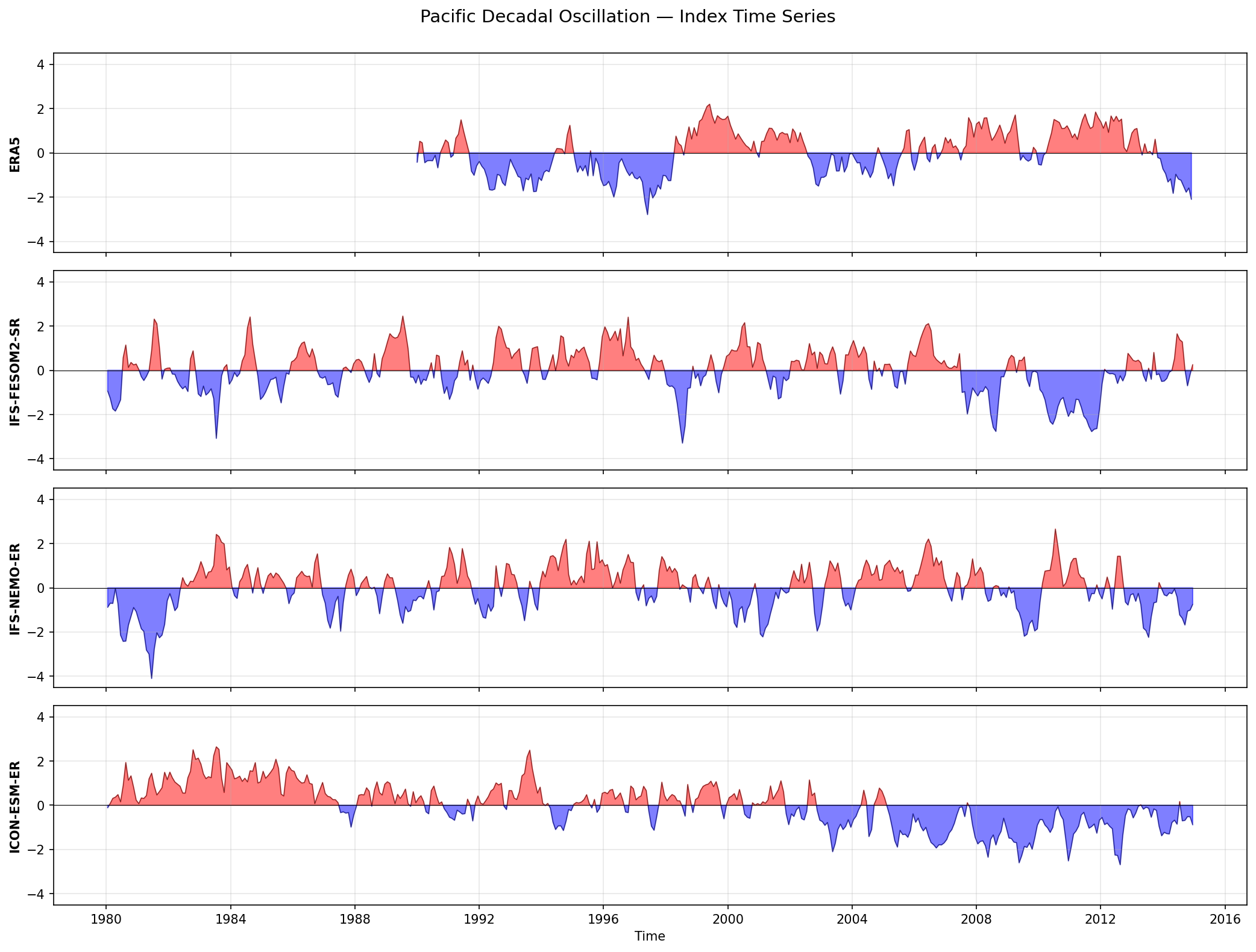
| Variables | tos |
|---|---|
| Models | IFS-FESOM2-SR, IFS-NEMO-ER, ICON-ESM-ER, HadGEM3-GC5 |
| Reference Dataset | ESA_CCI |
| Units | K |
| Period | 1980–2014 |
| IFS-FESOM2-SR | Std: 1.00 · Mean: -0.00 |
| IFS-NEMO-ER | Std: 1.00 · Mean: -0.00 |
| ICON-ESM-ER | Std: 1.00 · Mean: 0.00 |
| HadGEM3-GC5 | Std: 1.00 · Mean: 0.00 |
Summary high
Time series of the standardized Pacific Decadal Oscillation (PDO) index from 1980 to 2014 comparing four high-resolution coupled models against an observational reference (labelled ERA5).
Key Findings
- As expected for free-running coupled climate models, the phases of the PDO are uncorrelated with observations and between models; the evaluation focuses on the temporal character (frequency and persistence) of the variability.
- ICON-ESM-ER exhibits the most pronounced decadal-scale persistence, characterised by extended regimes of a single phase (e.g., positive 1980–1988, negative 2008–2012) compared to other models.
- IFS-FESOM2-SR and IFS-NEMO-ER show higher-frequency variability with more frequent sign switching, suggesting a less 'red' spectrum than ICON-ESM-ER.
- The observational record (top panel) appears truncated or missing prior to ~1989 in this specific plot.
Spatial Patterns
N/A (Temporal analysis). The figure displays temporal evolution where ICON-ESM-ER shows longer decorrelation timescales (multi-year persistence) compared to the more interannually variable IFS-based models.
Model Agreement
Models diverge in phase (expected due to internal variability) and show moderate diversity in the spectral character of the oscillation. ICON-ESM-ER stands out for having the most stable decadal regimes, while IFS variants appear more dominated by interannual frequencies.
Physical Interpretation
The PDO is physically associated with ocean memory and the integration of stochastic atmospheric forcing (red noise). The stronger persistence in ICON-ESM-ER suggests either greater upper-ocean thermal inertia or stronger coupled feedbacks sustaining the mode compared to the IFS and HadGEM3 configurations. The higher frequency switching in IFS models may indicate a dominance of ENSO-like interannual forcing over decadal ocean dynamics.
Caveats
- The 35-year analysis period (1980–2014) is very short for evaluating multidecadal variability (PDO period ~20–30 years), capturing at most 1–1.5 cycles.
- Observational data is missing for the first decade (1980–1989), limiting the comparison of regime duration.
- Indices are standardized (std=1.0), so raw SST anomaly magnitudes cannot be compared.
Quasi-Biennial Oscillation — Spatial Pattern
| Variables | ua |
|---|---|
| Models | IFS-FESOM2-SR, IFS-NEMO-ER, ICON-ESM-ER |
| Reference Dataset | ERA5 |
| Units | m/s |
| Period | 1980–2014 |
Summary high
The figure is a placeholder explicitly stating 'No spatial pattern for Quasi-Biennial Oscillation', indicating that horizontal spatial maps are not generated for this specific diagnostic.
Key Findings
- The figure contains no data or model output for IFS-FESOM2-SR, IFS-NEMO-ER, or ICON-ESM-ER.
- No spatial comparison against ERA5 is available in this specific panel.
- The diagnostic tool likely excludes horizontal spatial patterns for the QBO, as this mode is primarily defined by vertical propagation in the equatorial stratosphere.
Spatial Patterns
None displayed.
Model Agreement
Cannot be assessed due to lack of data.
Physical Interpretation
The Quasi-Biennial Oscillation (QBO) is characterized by alternating easterly and westerly wind regimes in the equatorial stratosphere that propagate downward over a period of ~28 months. Unlike surface-based teleconnections (e.g., NAO, PDO) which are effectively captured by 2D horizontal maps of pressure or temperature, the QBO is physically a vertical profile phenomenon. It is standardly diagnosed using time-height sections of zonal mean zonal wind or indices at specific pressure levels (e.g., 30 hPa or 50 hPa), which explains why a generic 'Spatial Pattern' map diagnostic might be disabled or considered uninformative for this specific mode.
Caveats
- The plot is a placeholder with no scientific content.
- Evaluation of QBO simulation quality requires alternative diagnostics (e.g., time series or Hovmoller diagrams).
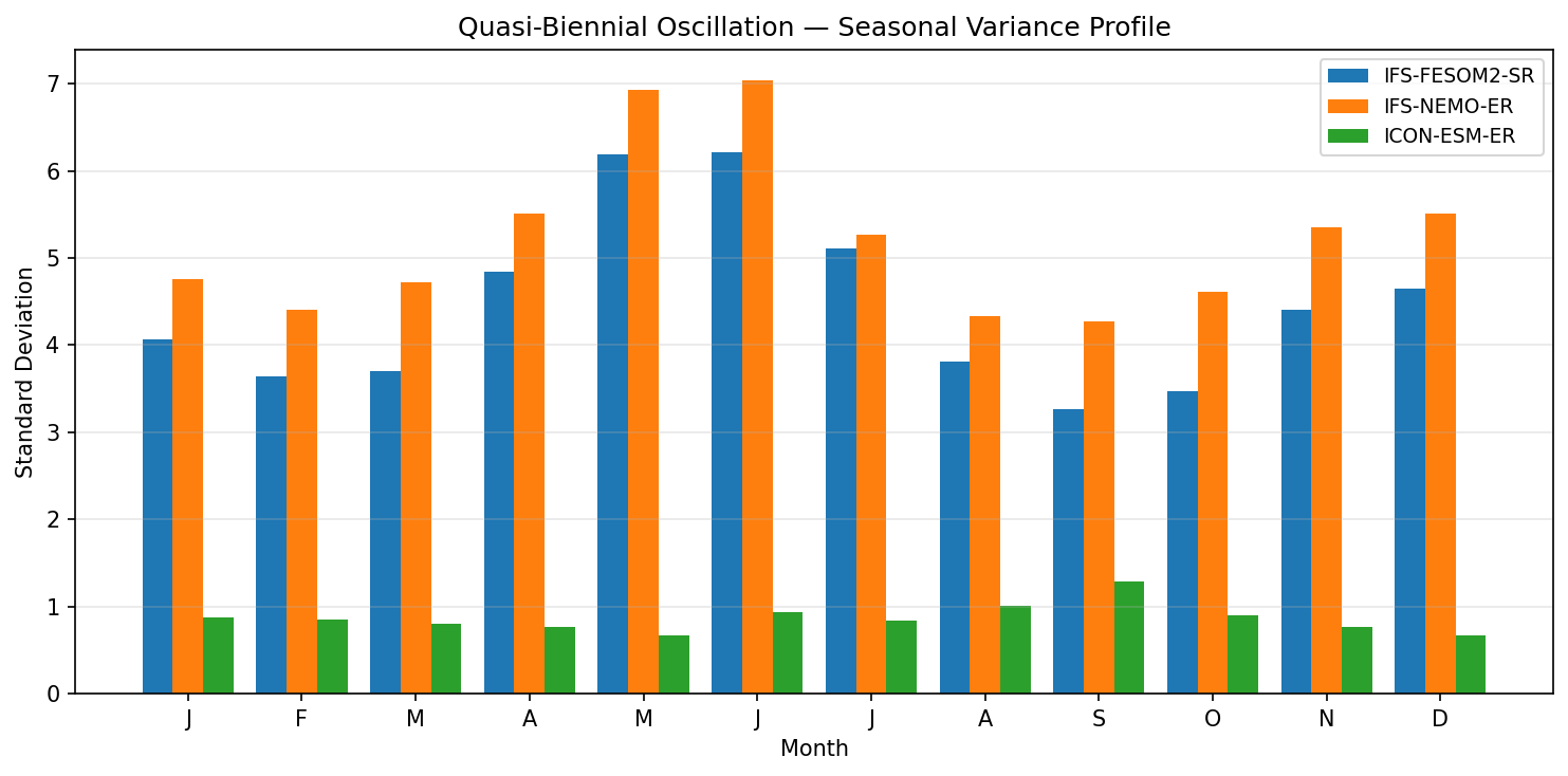
Quasi-Biennial Oscillation — Seasonal Variance Profile
| Variables | ua |
|---|---|
| Models | IFS-FESOM2-SR, IFS-NEMO-ER, ICON-ESM-ER |
| Reference Dataset | ERA5 |
| Units | m/s |
| Period | 1980–2014 |
| IFS-FESOM2-SR | Peak Month: 6.00 · Peak Std: 6.22 · Annual Std: 4.55 |
| IFS-NEMO-ER | Peak Month: 6.00 · Peak Std: 7.04 · Annual Std: 5.30 |
| ICON-ESM-ER | Peak Month: 9.00 · Peak Std: 1.29 · Annual Std: 0.88 |
Summary high
This figure displays the seasonal cycle of the standard deviation of the Quasi-Biennial Oscillation (QBO) index for three coupled models. The two IFS-based models exhibit significant variability with a pronounced seasonal cycle peaking in boreal summer, whereas ICON-ESM-ER shows negligible variability, indicating a failure to represent the QBO.
Key Findings
- ICON-ESM-ER fails to simulate a QBO, with a standard deviation consistently below 1.3 m/s, which is essentially noise compared to typical stratospheric wind variability.
- IFS-NEMO-ER exhibits the strongest QBO variability among the models, with an annual mean standard deviation of ~5.3 m/s and a peak of ~7.0 m/s in June.
- IFS-FESOM2-SR shows a similar seasonal phase to IFS-NEMO-ER (peaking in May/June) but with systematically lower amplitude (annual mean ~4.5 m/s).
- Both IFS models show a distinct seasonal modulation of QBO variance, with maximum variability in May-June and minima in September-October.
Spatial Patterns
While this is a temporal analysis, the seasonal profile reveals a structural dependence in the IFS models where variance is highest in boreal summer (May-July) and lowest in early autumn (September-October). This seasonality suggests a modulation of the QBO wave forcing or interaction with the Semi-Annual Oscillation (SAO).
Model Agreement
There is a strong dichotomy: the IFS-based models agree on the presence of the oscillation and the phase of its seasonal variance modulation, though they differ by ~15% in amplitude. In contrast, ICON-ESM-ER disagrees completely, effectively flatlining with no meaningful stratospheric oscillation.
Physical Interpretation
The QBO is driven by the upward propagation and dissipation of atmospheric waves (gravity, Kelvin, and Rossby-gravity waves). The failure of ICON-ESM-ER suggests insufficient vertical resolution in the stratosphere or inadequate non-orographic gravity wave parameterization to drive the oscillation. The higher variability in IFS-NEMO-ER compared to IFS-FESOM2-SR may reflect differences in atmospheric resolution (if the 'ER' configuration implies higher resolution than 'SR') or ocean-atmosphere coupling effects influencing wave generation sources.
Caveats
- No observational reference (e.g., ERA5) is plotted, preventing assessment of which IFS model is closer to reality in terms of absolute amplitude.
- The metadata identifies the observation variable as 'u10' (10m wind), which is likely a metadata error as QBO is a stratospheric phenomenon; this analysis assumes the plot correctly shows stratospheric zonal wind variability.
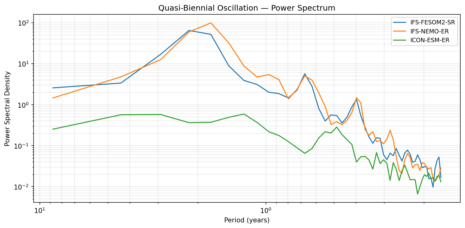
Quasi-Biennial Oscillation — Power Spectrum
| Variables | ua |
|---|---|
| Models | IFS-FESOM2-SR, IFS-NEMO-ER, ICON-ESM-ER |
| Reference Dataset | ERA5 |
| Units | m/s |
| Period | 1980–2014 |
Summary high
The power spectrum analysis reveals that both IFS-based models successfully generate a Quasi-Biennial Oscillation (QBO) with a realistic period, whereas ICON-ESM-ER fails to produce any significant stratospheric oscillation.
Key Findings
- IFS-NEMO-ER and IFS-FESOM2-SR exhibit a prominent spectral peak between 2 and 3 years, consistent with the observed ~28-month (2.33-year) QBO period.
- ICON-ESM-ER shows negligible power spectral density (2 orders of magnitude lower than IFS) and lacks a spectral peak in the QBO band, indicating the absence of a QBO.
- IFS-NEMO-ER displays slightly higher peak power than IFS-FESOM2-SR, though both IFS configurations agree on the fundamental frequency.
- Secondary peaks around 1 year suggest some annual cycle influence or harmonics in the IFS models, but the interannual QBO signal is dominant.
Spatial Patterns
This is a frequency-domain diagnostic. The temporal pattern for IFS models is dominated by a quasi-biennial periodicity (peak ~2.3 years), while ICON-ESM-ER exhibits a spectrum characteristic of noise or weak variability without preferred timescales in the interannual range.
Model Agreement
There is a stark dichotomy: the two IFS-based coupled models agree strongly and reproduce the phenomenon, while the ICON-ESM-ER model diverges completely by failing to simulate the oscillation. No observational line is plotted, but IFS performance aligns with theoretical expectations.
Physical Interpretation
The QBO is driven by wave-mean flow interactions involving Kelvin, Rossby-gravity, and small-scale gravity waves propagating up from the troposphere. The success of the IFS models implies sufficient vertical resolution in the stratosphere and/or effective non-orographic gravity wave drag parameterization. The failure of ICON-ESM-ER suggests insufficient vertical spacing or lacking gravity wave forcing needed to spontaneously generate and sustain the westerly/easterly phase transitions.
Caveats
- The observational reference (ERA5) mentioned in metadata is missing from the plot, preventing a quantitative assessment of amplitude bias relative to reality.
- The analysis relies on theoretical knowledge of the QBO period (~28 months) for validation in the absence of an observational curve.
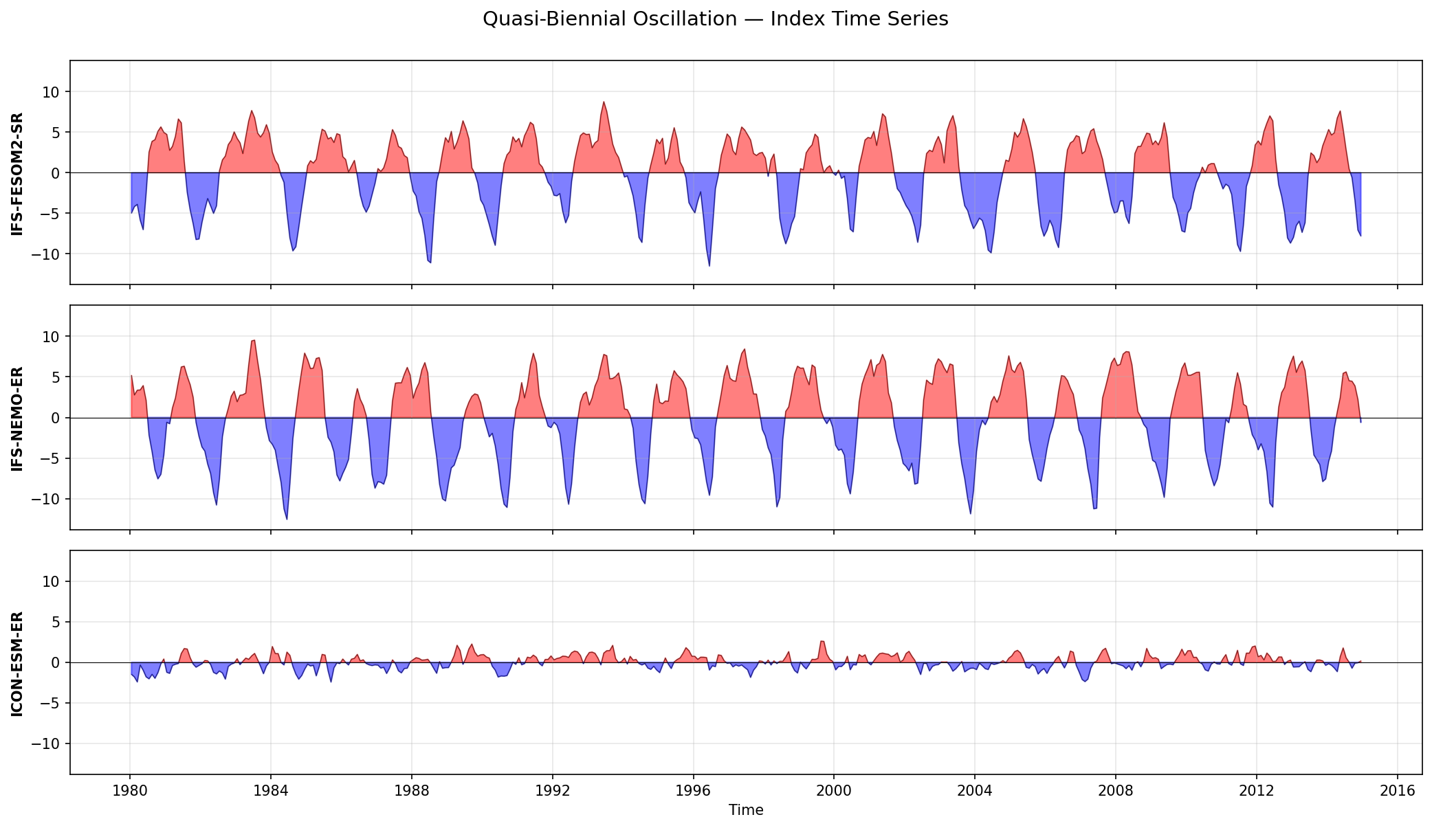
Quasi-Biennial Oscillation — Index Time Series
| Variables | ua |
|---|---|
| Models | IFS-FESOM2-SR, IFS-NEMO-ER, ICON-ESM-ER |
| Reference Dataset | ERA5 |
| Units | m/s |
| Period | 1980–2014 |
| IFS-FESOM2-SR | Std: 4.55 · Mean: -0.00 |
| IFS-NEMO-ER | Std: 5.30 · Mean: 0.00 |
| ICON-ESM-ER | Std: 0.88 · Mean: 0.00 |
Summary high
This diagnostic figure compares the time evolution of the Quasi-Biennial Oscillation (QBO) index across three models, revealing a successful simulation of the phenomenon in the IFS-based models but a complete absence in ICON-ESM-ER.
Key Findings
- IFS-FESOM2-SR and IFS-NEMO-ER simulate a robust QBO with realistic periodicity (~28 months) and amplitudes typically ranging between ±5 and ±12 m/s.
- ICON-ESM-ER fails to generate a QBO, exhibiting only weak, high-frequency fluctuations (standard deviation ~0.9 m/s) with no coherent quasi-biennial cycle.
- The IFS models capture the characteristic asymmetry of the QBO, with easterly phases (negative, blue) often reaching sharper and deeper peaks than the westerly phases (positive, red).
Spatial Patterns
IFS models show regular, alternating phases of stratospheric westerlies and easterlies persisting for roughly 2.3 years per cycle. ICON-ESM-ER lacks this temporal structure entirely.
Model Agreement
There is high consistency between the two IFS variants (FESOM2 vs NEMO ocean coupling), suggesting the QBO is robustly determined by the shared IFS atmospheric component. There is strong disagreement between the IFS models and ICON-ESM-ER.
Physical Interpretation
The QBO is driven by wave-mean flow interactions involving vertically propagating gravity, Kelvin, and Rossby-gravity waves. The success of the IFS models indicates sufficient stratospheric vertical resolution and effective non-orographic gravity wave drag parameterization. ICON-ESM-ER's failure implies insufficient vertical resolution or untuned gravity wave forcing mechanisms necessary to spontaneously drive the oscillation.
Caveats
- An observational reference line (e.g., ERA5) is not overlaid, precluding a direct phase and amplitude validation, though IFS behavior is qualitatively realistic.
- The specific pressure level defining the index (typically 50 hPa or 30 hPa) is not labeled, though the dynamics shown are standard for the lower stratosphere.
Southern Annular Mode — Spatial Pattern
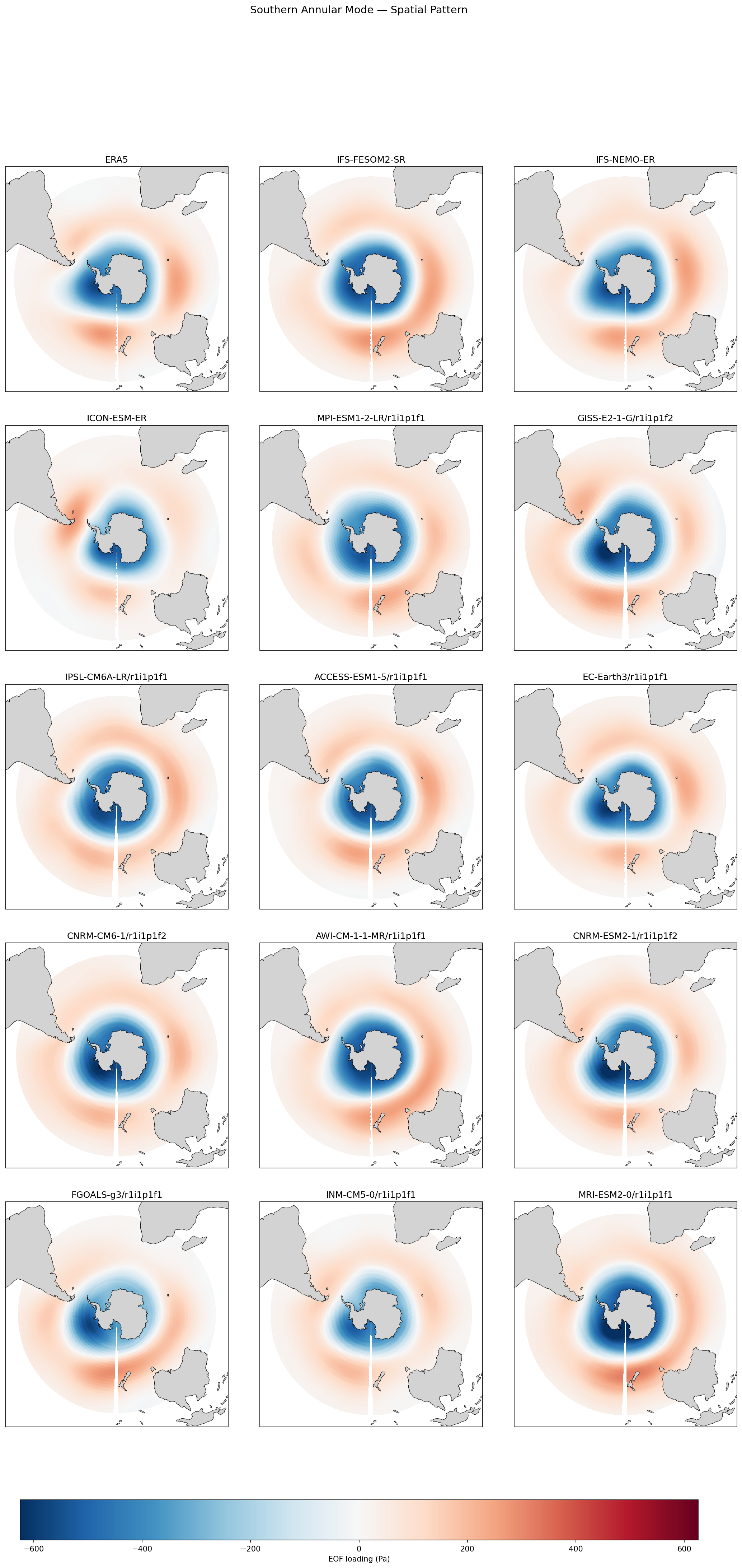
| Variables | psl |
|---|---|
| Models | IFS-FESOM2-SR, IFS-NEMO-ER, ICON-ESM-ER |
| Reference Dataset | ERA5 |
| Units | Pa |
| Period | 1980–2014 |
| IFS-FESOM2-SR | Variance Explained: 0.37 |
| IFS-NEMO-ER | Variance Explained: 0.30 |
| ICON-ESM-ER | Variance Explained: 0.25 |
| ERA5 | Variance Explained: 0.27 |
Summary high
This figure displays the spatial pattern (EOF1 of sea level pressure) of the Southern Annular Mode (SAM) for ERA5 reanalysis, three high-resolution EERIE models, and a selection of CMIP6 models. It compares the characteristic dipole structure—low pressure over Antarctica surrounded by a mid-latitude high-pressure ring—and the fraction of variance explained by this mode.
Key Findings
- All three EERIE models (IFS-FESOM2-SR, IFS-NEMO-ER, ICON-ESM-ER) successfully reproduce the classic annular structure of the SAM, with a negative pressure anomaly over the polar cap and a positive anomaly belt at ~40–50°S.
- IFS-NEMO-ER shows excellent agreement with ERA5 in terms of mode dominance, explaining 29.9% of the variance compared to ERA5's 27.3%.
- IFS-FESOM2-SR overestimates the dominance of the SAM, explaining 36.5% of the total variance, suggesting the mode is too regular or other variability is suppressed relative to observations.
- ICON-ESM-ER slightly underestimates the variance explained (25.1%) and displays a marginally weaker spatial loading pattern compared to the IFS simulations.
Spatial Patterns
The observed pattern in ERA5 features a deep negative pressure loading (<-400 Pa) centred over Antarctica and a positive loading ring in the mid-latitudes, consistent with a strengthening of the westerlies. The EERIE models capture the zonal asymmetry of the positive ring well (e.g., breaks/weakening in the Pacific sector). The CMIP6 models generally show similar patterns, though with varying intensities; for example, INM-CM5-0 and FGOALS-g3 show notably weaker amplitude loadings compared to the high-resolution models.
Model Agreement
There is high structural agreement between the EERIE models and ERA5. The primary divergence is in the amplitude of the loading and the variance explained. IFS-NEMO-ER provides the closest match to the ERA5 benchmark. The EERIE models appear comparable to the better-performing CMIP6 models (e.g., ACCESS-ESM1-5, MPI-ESM1-2-LR) and avoid the weak pattern definition seen in some lower-resolution CMIP6 members (e.g., FGOALS-g3).
Physical Interpretation
The SAM represents the north-south vacillation of the Southern Hemisphere eddy-driven jet. The correct simulation of this spatial pattern implies the models are effectively resolving the storm tracks and the wave-mean flow interactions that maintain the jet. The high variance explained in IFS-FESOM2-SR might indicate a jet that is too persistent or zonally symmetric, whereas the values closer to 27% (ERA5/IFS-NEMO-ER) reflect a more realistic balance between the SAM and other modes of variability.
Caveats
- Variance explained is sensitive to the exact domain and pre-processing (detrending/deseasonalising) used.
- The analysis does not show the temporal evolution or index, preventing assessment of trends or seasonality.
Southern Annular Mode — Seasonal Variance Profile
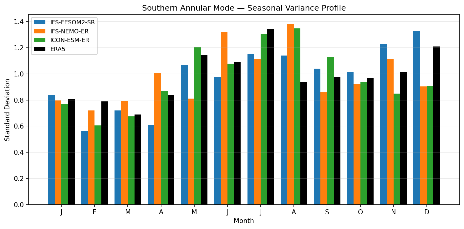
| Variables | psl |
|---|---|
| Models | IFS-FESOM2-SR, IFS-NEMO-ER, ICON-ESM-ER |
| Reference Dataset | ERA5 |
| Units | Pa |
| Period | 1980–2014 |
| IFS-FESOM2-SR | Peak Month: 12.00 · Peak Std: 1.33 · Annual Std: 1.00 |
| IFS-NEMO-ER | Peak Month: 8.00 · Peak Std: 1.38 · Annual Std: 1.00 |
| ICON-ESM-ER | Peak Month: 8.00 · Peak Std: 1.35 · Annual Std: 1.00 |
Summary high
This figure evaluates the seasonal cycle of Southern Annular Mode (SAM) variability by comparing the monthly standard deviation of the SAM index in three high-resolution models against ERA5 reanalysis. While models generally capture the range of variability, they exhibit significant discrepancies in the timing and duration of peak variance, particularly during the austral winter and summer.
Key Findings
- ERA5 shows a distinct primary peak in SAM variability in July (~1.35 standard deviations) and a secondary increase in December (~1.2).
- ICON-ESM-ER captures the magnitude of the July peak well but erroneously sustains high variability into August and September, failing to reproduce the observed sharp decline.
- IFS-NEMO-ER displays a noisy seasonal cycle with a delayed peak in August (~1.38) and underestimates the December variability.
- IFS-FESOM2-SR misses the austral winter peak (underestimating July-August) but produces the strongest austral summer variability, peaking in December (~1.33).
Spatial Patterns
The observational baseline (ERA5) indicates a seasonal modulation where SAM variance is highest in mid-winter (July) and early summer (December), with relative lulls in spring and autumn. The models struggle to replicate this double-peak structure, often smoothing it out or shifting the phase.
Model Agreement
Inter-model agreement is low regarding the specific shape of the seasonal cycle. ICON-ESM-ER and IFS-NEMO-ER tend to overestimate variability in late winter (August), while IFS-FESOM2-SR behaves differently, focusing its energy in the summer (December). None of the models perfectly replicate the ERA5 July peak followed by an August dip.
Physical Interpretation
SAM variability is driven by internal atmospheric dynamics (eddy-mean flow interactions) and modulated by the stratospheric polar vortex. The winter peak relates to the dynamics of the strengthened jet stream, while the summer peak (Nov-Dec) is often influenced by stratosphere-troposphere coupling (e.g., vortex breakdown). The delayed or sustained peaks in ICON and IFS-NEMO suggest biases in the seasonal evolution of the SH eddy-driven jet or persistent sea ice feedbacks, while IFS-FESOM2-SR's December peak may indicate a stronger or more sensitive stratospheric coupling in summer.
Caveats
- The indices appear to be normalized to unit annual standard deviation, meaning the plot assesses the relative seasonal distribution of variance rather than absolute amplitude differences.
- The analysis period (1980-2014) includes the ozone hole era, which strongly influences SAM trends and variability in austral summer; model representation of ozone chemistry is a potential confounding factor.
Southern Annular Mode — Power Spectrum
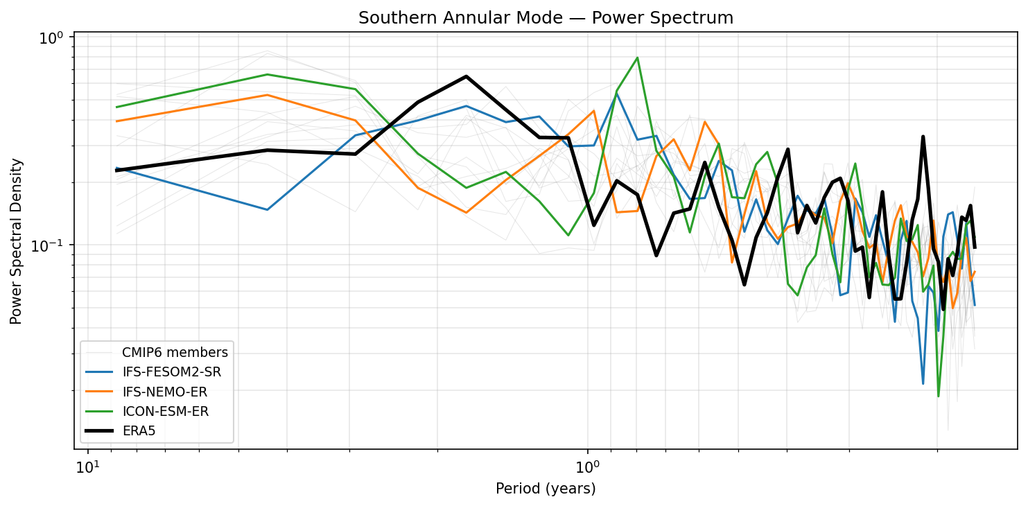
| Variables | psl |
|---|---|
| Models | IFS-FESOM2-SR, IFS-NEMO-ER, ICON-ESM-ER |
| Reference Dataset | ERA5 |
| Units | Pa |
| Period | 1980–2014 |
Summary medium
This figure displays the power spectral density of the Southern Annular Mode (SAM) index for three high-resolution models compared to ERA5 reanalysis and the CMIP6 ensemble. The analysis assesses how well models capture the temporal variability timescales of the SAM, characterized generally by a red noise spectrum.
Key Findings
- All models and ERA5 exhibit a general 'red noise' spectrum, with power increasing as the period lengthens, consistent with the expected persistence of the SAM.
- ICON-ESM-ER shows a distinct, anomalous sharp spectral peak at a period of approximately 1.2 years, which is not present in ERA5 or the IFS models.
- IFS-NEMO-ER and ICON-ESM-ER overestimate variability at decadal timescales (periods > 5 years) relative to ERA5, although they remain within the broad spread of the CMIP6 ensemble.
- IFS-FESOM2-SR shows the best agreement with ERA5 in the interannual band (2–5 years), closely tracking the observed spectral density magnitude and shape.
Spatial Patterns
Not applicable (temporal spectrum). The dominant temporal feature is the inverse relationship between frequency and power (red noise).
Model Agreement
The models broadly agree on the spectral slope but diverge in specific frequency bands. At low frequencies (>5 years), the spread is large (consistent with CMIP6). At interannual scales, IFS-FESOM2-SR aligns best with observations, while ICON-ESM-ER introduces a spurious quasi-periodic signal near 1 year.
Physical Interpretation
The SAM is an internal mode of atmospheric variability with a timescale reddened by interactions with the ocean and cryosphere. The broad agreement on the spectral slope suggests models capture the fundamental eddy-mean flow feedbacks. The excess power at low frequencies in NEMO/ICON runs may imply stronger-than-observed ocean coupling or persistence. The sharp peak in ICON near the annual cycle suggests potential issues with seasonal cycle removal or a resonant interaction not seen in reality.
Caveats
- The analysis period (1980–2014, 35 years) is short for robustly estimating power spectral density at decadal timescales (left side of the plot).
- The CMIP6 spread is very wide at low frequencies, indicating high internal variability or model uncertainty in decadal SAM dynamics.
Southern Annular Mode — Index Time Series
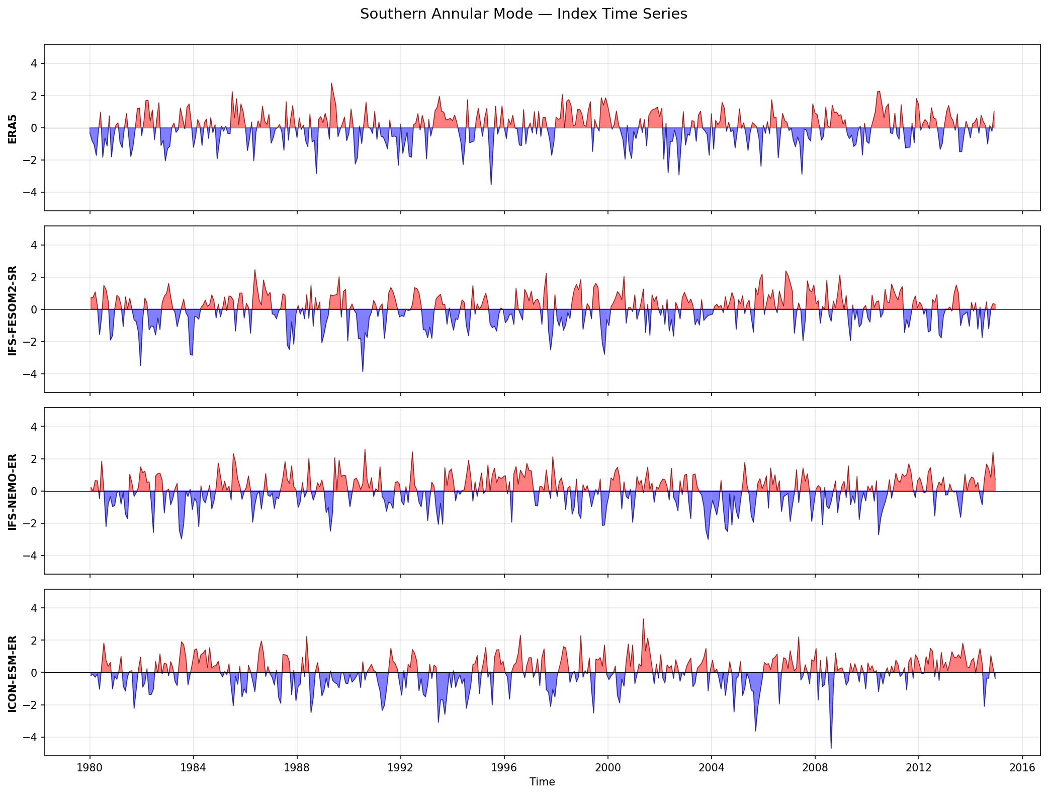
| Variables | psl |
|---|---|
| Models | IFS-FESOM2-SR, IFS-NEMO-ER, ICON-ESM-ER |
| Reference Dataset | ERA5 |
| Units | Pa |
| Period | 1980–2014 |
| IFS-FESOM2-SR | Std: 1.00 · Mean: 0.00 |
| IFS-NEMO-ER | Std: 1.00 · Mean: 0.00 |
| ICON-ESM-ER | Std: 1.00 · Mean: 0.00 |
Summary high
The figure presents the monthly time series of the Southern Annular Mode (SAM) index from 1980 to 2014 for ERA5 reanalysis and three high-resolution coupled models (IFS-FESOM2-SR, IFS-NEMO-ER, ICON-ESM-ER), illustrating the temporal variability of the Southern Hemisphere's dominant climate mode.
Key Findings
- All three models successfully reproduce the stochastic, noisy character of the SAM index observed in ERA5, with no evidence of pathological periodicities or locking behavior.
- The dynamic range of the indices is consistent across models and observations, with typical fluctuations within ±2 standard deviations and occasional extreme events exceeding ±3 (e.g., ICON-ESM-ER around 2001, ERA5 around 1999).
- The persistence of positive and negative phases (the 'redness' of the time series) appears visually similar between the models and ERA5, indicating realistic autocorrelation timescales.
- No strong long-term trend is immediately visually apparent in the model time series over this 35-year period, which is dominated by high-frequency internal variability.
Spatial Patterns
While the figure shows temporal data, the time series exhibit characteristic red noise behavior: rapid month-to-month fluctuations superimposed on interannual variability. There is no regular seasonal locking or distinct periodicity, consistent with the SAM being an internal mode of atmospheric variability driven by eddy-mean flow interactions.
Model Agreement
The models show excellent agreement with ERA5 in terms of the statistical properties of the time series (variance, amplitude, and frequency of sign changes). As these are free-running coupled simulations, the specific timing of El Niño/La Niña-like influences or specific SAM events does not synchronize with the historical ERA5 record, which is expected behavior.
Physical Interpretation
The SAM represents the north-south vacillation of the eddy-driven westerly jet in the Southern Hemisphere. The realistic temporal structure suggests that the high-resolution models (IFS and ICON variants) correctly capture the stochastic forcing of the zonal flow by synoptic-scale eddies. The absence of unrealistic persistence implies that the negative feedbacks (frictional damping, eddy feedback) regulating the jet's position are operating correctly.
Caveats
- The indices are standardized (mean=0, std=1), which masks any systematic biases in the absolute position or strength of the Southern Hemisphere westerlies.
- The 35-year period is relatively short for detecting forced long-term trends (e.g., the positive SAM trend associated with ozone depletion and GHG increases) against the background of strong internal variability.