Sea Ice Sea Ice CMIP6
CMIP6 Multi-Model Mean Context
Comparison with CMIP6 ensemble mean from 7 members.
Contributing models: ACCESS-ESM1-5, CNRM-CM6-1, CNRM-ESM2-1, EC-Earth3, INM-CM5-0, MPI-ESM1-2-LR, MRI-ESM2-0
Synthesis
Related diagnostics
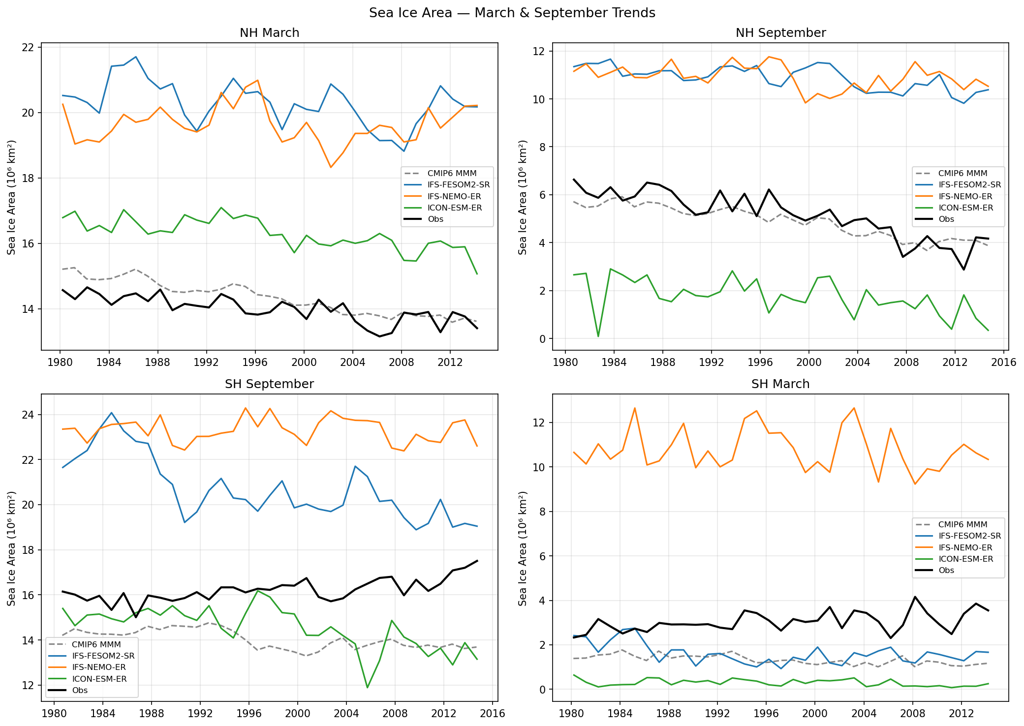
Sea Ice Area March & September Trends
| Variables | siconc, sithick |
|---|---|
| Models | MPI-ESM1-2-LR, ACCESS-ESM1-5, EC-Earth3, CNRM-CM6-1, CNRM-ESM2-1, INM-CM5-0, MRI-ESM2-0, IFS-FESOM2-SR, IFS-NEMO-ER, ICON-ESM-ER, HadGEM3-GC5 |
| Reference Dataset | OSI_SAF |
| Units | 0-1 |
| Period | 1980–2014 |
Summary high
This figure evaluates annual maximum and minimum sea ice area trends for the Northern and Southern Hemispheres, revealing severe biases in the high-resolution EERIE models compared to observations (OSI-SAF) and the CMIP6 multi-model mean. The IFS variants generally suffer from massive positive biases (too much ice), while ICON-ESM-ER exhibits exaggerated seasonality in the Arctic and general underestimation in the Antarctic.
Key Findings
- IFS-NEMO-ER and IFS-FESOM2-SR grossly overestimate NH sea ice area in both March and September by ~5-6 million km², placing their summer minimums (~11 million km²) well above the observed winter maximums in some years.
- IFS-NEMO-ER shows a catastrophic positive bias in the Antarctic summer (SH March), retaining over 10 million km² of ice compared to observations of ~3 million km², indicating a failure of seasonal melt.
- ICON-ESM-ER displays an amplified seasonal cycle in the NH: it overestimates the March maximum by ~2 million km² but severely underestimates the September minimum, approaching ice-free conditions (<2 million km²) well below observations.
- The CMIP6 Multi-Model Mean (MMM) tracks observations significantly better than the specific high-resolution simulations shown, particularly capturing the absolute magnitude and downward trend of NH September sea ice.
Spatial Patterns
The IFS biases manifest as large systematic offsets (roughly +6 million km² in NH) rather than trend errors. In the SH, IFS-FESOM2-SR exhibits a notable 'drift' or regime shift around 1988 in September, dropping from ~23 to ~19 million km², suggesting initialization shock. ICON-ESM-ER is consistently low in the SH.
Model Agreement
There is very poor agreement among models and with observations. The spread between models is extreme, exceeding 8 million km² in SH March—larger than the observational mean itself. The high-resolution models do not converge toward the CMIP6 baseline.
Physical Interpretation
The pervasive positive bias in IFS models suggests a strong cold bias in the atmosphere/ocean or incorrect sea ice albedo parameterizations preventing summer melt. The ICON pattern (excessive winter area, deficient summer area) implies the formation of extensive but thermodynamically thin ice that melts too easily. The IFS-FESOM drift implies the ocean state was still adjusting (spin-up) during the first decade of the run.
Caveats
- The extreme magnitude of biases (especially IFS-NEMO-ER in SH) suggests these specific model tunings are physically unrealistic for polar cryosphere studies.
- Drift in IFS-FESOM2-SR indicates the simulation may not be in equilibrium.
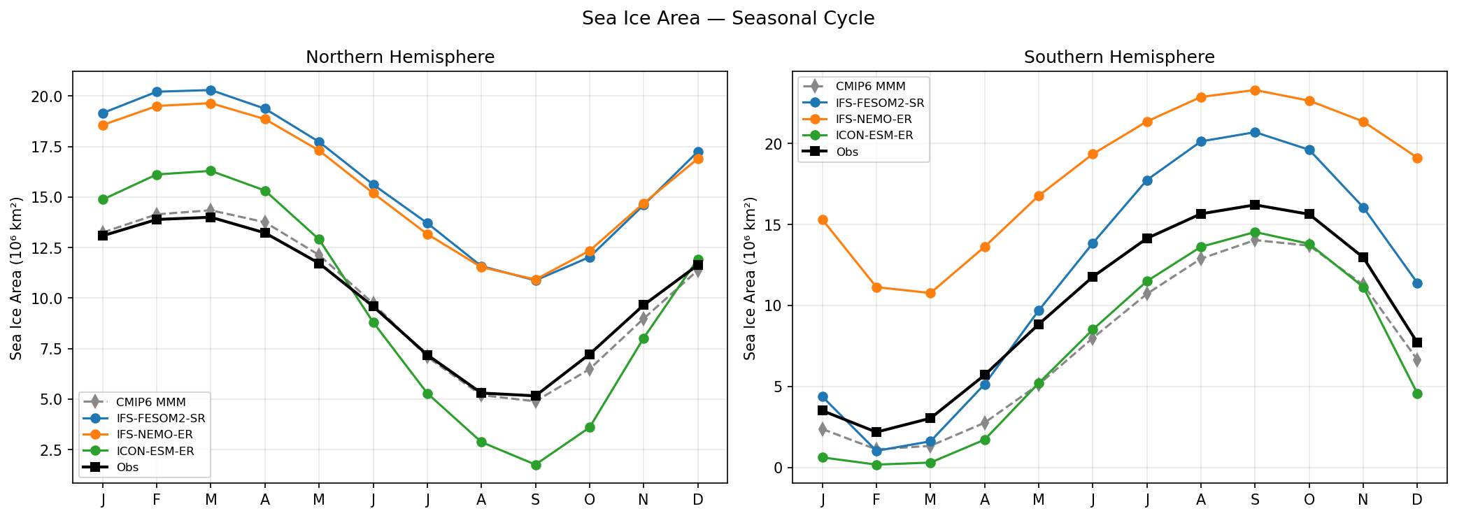
Sea Ice Area Seasonal Cycle
| Variables | siconc, sithick |
|---|---|
| Models | MPI-ESM1-2-LR, ACCESS-ESM1-5, EC-Earth3, CNRM-CM6-1, CNRM-ESM2-1, INM-CM5-0, MRI-ESM2-0, IFS-FESOM2-SR, IFS-NEMO-ER, ICON-ESM-ER, HadGEM3-GC5 |
| Reference Dataset | OSI_SAF |
| Units | 0-1 |
| Period | 1980–2014 |
Summary high
This diagnostic compares the seasonal cycle of Northern and Southern Hemisphere sea ice area from three high-resolution EERIE models against OSI-SAF observations and the CMIP6 multi-model mean. The models exhibit drastic biases: IFS configurations show massive overestimations of sea ice area, while ICON-ESM-ER tends to exaggerate seasonal amplitude in the North and underestimate area in the South.
Key Findings
- IFS-NEMO-ER and IFS-FESOM2-SR exhibit a severe, systematic positive bias in the Northern Hemisphere (NH), overestimating sea ice area by ~6 million km² year-round; their summer minimum (~11 million km²) is more than double the observed value (~5 million km²).
- In the Southern Hemisphere (SH), IFS-NEMO-ER maintains a huge positive bias throughout the year (+5 to +9 million km²). IFS-FESOM2-SR shows a similar winter overshoot but agrees well with observations during the summer minimum.
- ICON-ESM-ER displays an exaggerated seasonal cycle in the NH, with too much winter ice (~16 vs 14 million km²) and a severe underestimation of summer ice (<2 vs 5 million km²).
- The CMIP6 MMM significantly outperforms the high-resolution IFS models in the NH, tracking observations closely, but underestimates SH winter maxima, a bias shared by ICON-ESM-ER.
Spatial Patterns
While the phasing (timing of minima/maxima) is generally captured correctly—March/September for NH and February/September for SH—the amplitudes differ. IFS models in the NH show correct amplitude (~9 million km²) but a massive mean-state offset. ICON-ESM-ER in the NH shows an excessive amplitude (~14 million km²).
Model Agreement
Inter-model agreement is poor. The two IFS models (differing in ocean discretization) generally cluster with high positive biases, though they diverge in the SH summer. ICON-ESM-ER behaves distinctly, resembling the CMIP6 MMM pattern in the SH (low bias) but deviating in the NH (strong seasonal cycle).
Physical Interpretation
The systematic positive offset in IFS models suggests a profound cold bias in the polar regions or issues with initial conditions/drift retaining too much ice; the lack of summer melt reduction implies albedo or cloud feedback issues. ICON-ESM-ER's deep NH summer melt suggests a too-strong ice-albedo feedback or initially thin ice. The low SH bias in ICON/CMIP6 is consistent with the common 'warm Southern Ocean' bias, whereas IFS appears to have a 'cold Southern Ocean' or excessive freezing bias.
Caveats
- Figure evaluates area only, not volume/thickness; models with excessive area might still have realistic or too-low volume if ice is very thin.
- Large biases suggest these runs might be in drift or have significant tuning imbalances in polar energy budgets.
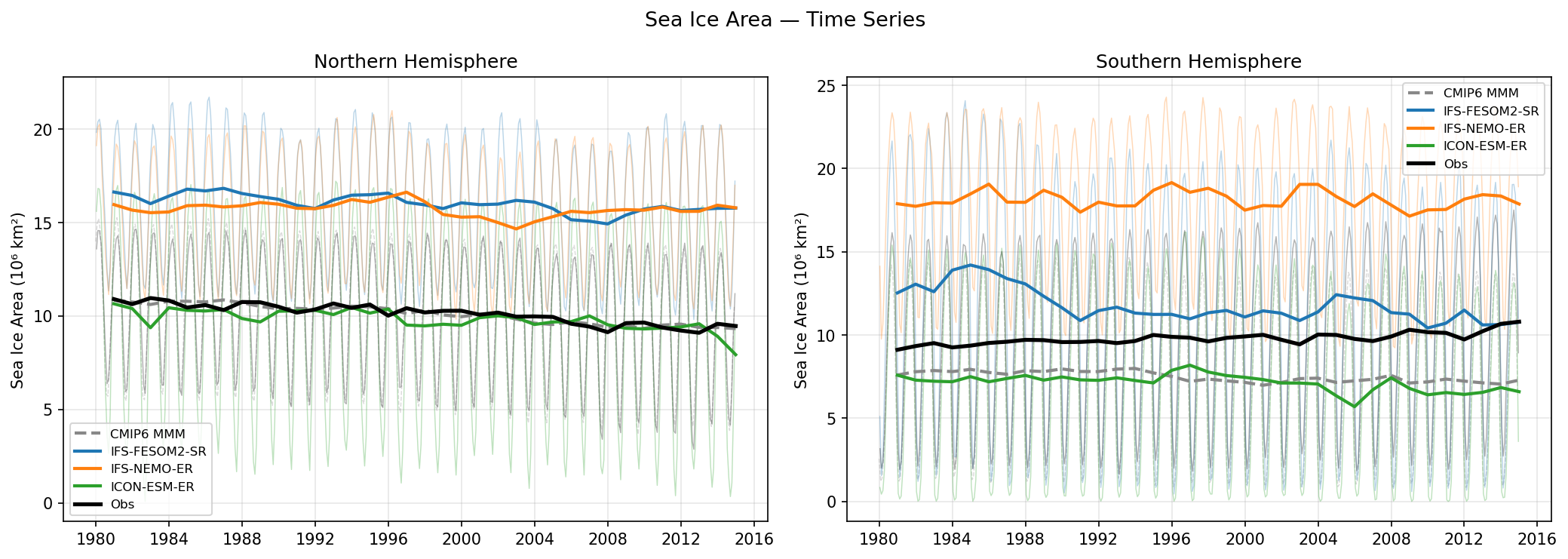
Sea Ice Area Time Series
| Variables | siconc, sithick |
|---|---|
| Models | MPI-ESM1-2-LR, ACCESS-ESM1-5, EC-Earth3, CNRM-CM6-1, CNRM-ESM2-1, INM-CM5-0, MRI-ESM2-0, IFS-FESOM2-SR, IFS-NEMO-ER, ICON-ESM-ER, HadGEM3-GC5 |
| Reference Dataset | OSI_SAF |
| Units | 0-1 |
| Period | 1980–2014 |
Summary high
Time series of Northern and Southern Hemisphere sea ice area (1980–2014) comparing three high-resolution models against OSI-SAF observations and the CMIP6 multi-model mean.
Key Findings
- ICON-ESM-ER shows excellent agreement with Northern Hemisphere (NH) observations, closely tracking the magnitude and negative trend of the CMIP6 MMM and OSI-SAF data.
- Both IFS-based models (IFS-FESOM2-SR and IFS-NEMO-ER) exhibit a massive positive bias in the NH, overestimating annual mean sea ice area by ~5-6 million km² (approx. 50% higher than observations).
- Southern Hemisphere (SH) results show large inter-model divergence: IFS-NEMO-ER drastically overestimates area (~18 vs 10 million km²), IFS-FESOM2-SR overestimates to a lesser degree, while ICON-ESM-ER underestimates area (~7 vs 10 million km²).
- IFS-FESOM2-SR displays a noticeable negative drift in the SH, decreasing from ~13 to ~11 million km² over the simulation period, suggesting equilibration issues.
Spatial Patterns
The Northern Hemisphere is characterized by a stable observational baseline with a slight decline, captured well by ICON but offset by a large constant bias in IFS models. The Southern Hemisphere shows high variability and stronger model disagreement, with IFS-NEMO-ER nearly doubling the observed ice area.
Model Agreement
Low inter-model agreement. The models cluster into two behaviors: ICON mimics the CMIP6 MMM (good NH, low SH), while the IFS family consistently predicts significantly more sea ice than observed in both hemispheres.
Physical Interpretation
The excessive sea ice in the IFS models suggests a systematic cold bias in high-latitude sea surface temperatures or aggressive sea ice formation/retention parameterizations. The underestimation of SH ice by ICON is a common feature in climate models (often linked to Warm Southern Ocean biases). The drift in IFS-FESOM2-SR SH ice implies the model is adjusting from its initial ocean state.
Caveats
- Sea ice area integrates concentration and extent but does not reveal thickness or volume errors.
- The analysis does not distinguish between summer minimum and winter maximum biases specifically, though the annual mean offset is dominant.
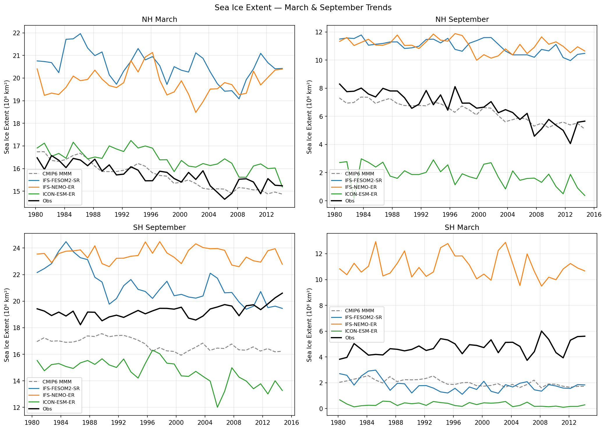
Sea Ice Extent March & September Trends
| Variables | siconc, sithick |
|---|---|
| Models | MPI-ESM1-2-LR, ACCESS-ESM1-5, EC-Earth3, CNRM-CM6-1, CNRM-ESM2-1, INM-CM5-0, MRI-ESM2-0, IFS-FESOM2-SR, IFS-NEMO-ER, ICON-ESM-ER, HadGEM3-GC5 |
| Reference Dataset | OSI_SAF |
| Units | 0-1 |
| Period | 1980–2014 |
Summary high
The figure evaluates annual sea ice extent trends in the Northern and Southern Hemispheres (March and September) for four high-resolution models against OSI-SAF observations and CMIP6 context. Model performance is highly variable; HadGEM3-GC5 excels in the Northern Hemisphere, while IFS-NEMO-ER and ICON-ESM-ER exhibit massive systematic biases—excessive ice and insufficient ice, respectively.
Key Findings
- HadGEM3-GC5 shows excellent agreement with observations in the NH, capturing both magnitude and the declining trend in March and September, though it significantly underestimates SH extent (e.g., ~6 million km² deficit in SH September).
- IFS-NEMO-ER exhibits a severe systematic positive bias globally, overestimating sea ice extent in all seasons and hemispheres (e.g., NH March ~21 vs. Obs ~16 million km²; SH March ~11 vs. Obs ~4 million km²).
- ICON-ESM-ER consistently underestimates sea ice, with critical failures in summer months; NH September is ~2 million km² (Obs ~6) and SH March is near-zero, indicating a nearly ice-free Antarctic summer.
- IFS-FESOM2-SR shares the large positive bias of IFS-NEMO in the NH and SH winter, but correctly switches to a low bias in SH summer (March), unlike the NEMO variant.
Spatial Patterns
The observed NH September decline is clearly visible in HadGEM3-GC5 and the CMIP6 MMM, whereas IFS models show little trend due to their biased high baselines. In the SH, models generally fail to capture the observed stability/slight increase, with baselines varying wildly from ~12 million km² (HadGEM3) to ~24 million km² (IFS-NEMO) for the winter maximum.
Model Agreement
Inter-model agreement is very poor, with models bracketing observations by large margins (up to 100% relative error in summer minima). The high-resolution models do not converge; instead, they show distinct, likely structural biases (IFS too cold/icy, ICON too warm/melt-prone).
Physical Interpretation
IFS-NEMO-ER's pervasive excessive ice suggests a global cold bias or overly aggressive ice formation/insufficient melt parametrization. ICON-ESM-ER's lack of summer ice suggests a strong warm bias or excessive albedo feedback sensitivity. HadGEM3-GC5's NH/SH dichotomy (good NH, low SH) is consistent with common biases in coupled models where Southern Ocean warming/cloud feedback errors lead to reduced Antarctic ice.
Caveats
- Analysis relies on extent only; ice volume or thickness biases might differ.
- The SH March bias in IFS-NEMO-ER is extreme (doubling the observed extent), suggesting a potential configuration or regridding error rather than just physical bias.
Sea Ice Extent Seasonal Cycle
| Variables | siconc, sithick |
|---|---|
| Models | MPI-ESM1-2-LR, ACCESS-ESM1-5, EC-Earth3, CNRM-CM6-1, CNRM-ESM2-1, INM-CM5-0, MRI-ESM2-0, IFS-FESOM2-SR, IFS-NEMO-ER, ICON-ESM-ER, HadGEM3-GC5 |
| Reference Dataset | OSI_SAF |
| Units | 0-1 |
| Period | 1980–2014 |
Summary high
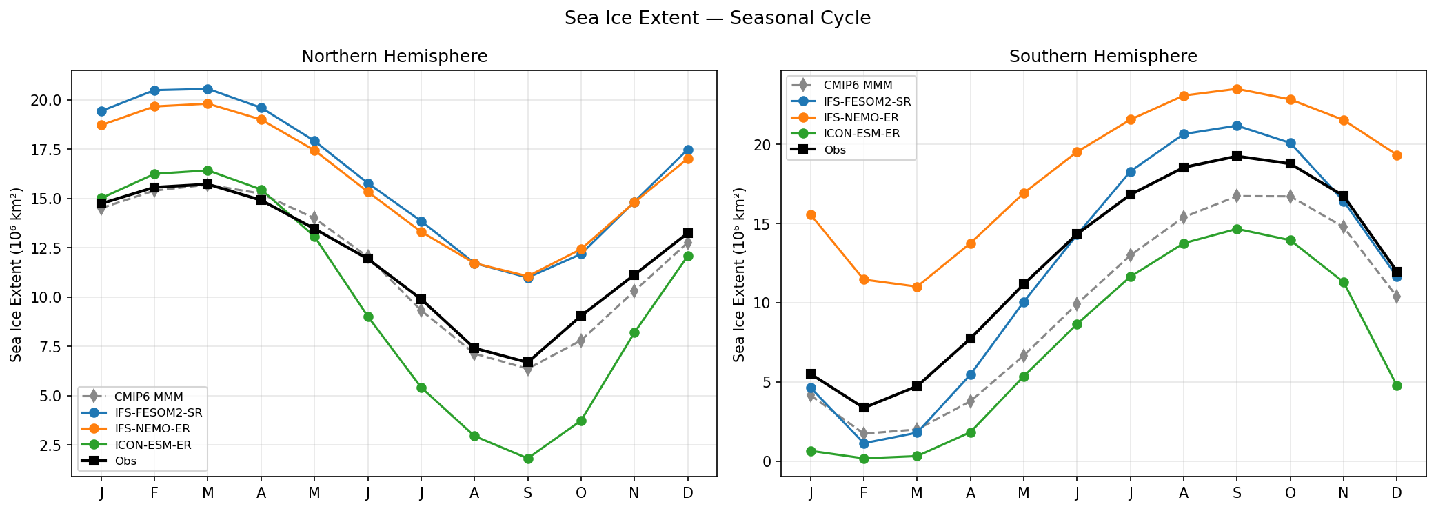
This figure evaluates the seasonal cycle of Northern and Southern Hemisphere sea ice extent for three high-resolution coupled models against OSI-SAF observations and the CMIP6 multi-model mean. The models exhibit large, divergent biases, with IFS variants generally overestimating extent and ICON-ESM-ER tending towards excessive melting, particularly in summer.
Key Findings
- IFS-FESOM2-SR and IFS-NEMO-ER show a systematic positive bias in the Northern Hemisphere, overestimating extent by ~4–5 × 10⁶ km² year-round compared to observations.
- ICON-ESM-ER captures the NH winter maximum well (~16 × 10⁶ km²) but suffers from extreme summer melt, dropping to <2 × 10⁶ km² in September (vs ~6.5 × 10⁶ km² in observations), implying a nearly ice-free summer Arctic.
- In the Southern Hemisphere, inter-model spread is extreme: IFS-NEMO-ER vastly overestimates ice (winter max >23 × 10⁶ km²), while ICON-ESM-ER severely underestimates it year-round (winter max <15 × 10⁶ km²).
Spatial Patterns
The seasonal phase is generally correct across models (maxima in March/September), but mean states differ fundamentally. The NH biases for IFS models are relatively constant offsets, whereas ICON shows a strong amplitude bias (correct winter, too low summer). In the SH, IFS-NEMO-ER fails to melt back sufficiently in summer (Feb), retaining ~11 × 10⁶ km² vs ~3.5 × 10⁶ km² observed.
Model Agreement
Inter-model agreement is very low, with spreads exceeding 50% of the mean value in some seasons. The CMIP6 MMM baseline often outperforms the individual high-resolution simulations, particularly in the NH where it tracks observations closely.
Physical Interpretation
The shared positive bias in NH for both IFS-based models suggests a common atmospheric driver (e.g., cold bias) or sea ice tuning that favors excessive growth/retention. Conversely, ICON-ESM-ER appears to have overly strong positive feedbacks (likely ice-albedo) or insufficient ocean stratification/too warm ocean temperatures, leading to rapid summer loss in the NH and inhibited growth in the SH.
Caveats
- Sea ice extent (area with >15% concentration) does not reflect ice thickness or volume, which might show different bias patterns.
- Observational uncertainty exists in melt ponds/summer retrieval, but model biases here (up to 5-10 million km²) far exceed instrument error.
Sea Ice Extent Time Series
| Variables | siconc, sithick |
|---|---|
| Models | MPI-ESM1-2-LR, ACCESS-ESM1-5, EC-Earth3, CNRM-CM6-1, CNRM-ESM2-1, INM-CM5-0, MRI-ESM2-0, IFS-FESOM2-SR, IFS-NEMO-ER, ICON-ESM-ER, HadGEM3-GC5 |
| Reference Dataset | OSI_SAF |
| Units | 0-1 |
| Period | 1980–2014 |
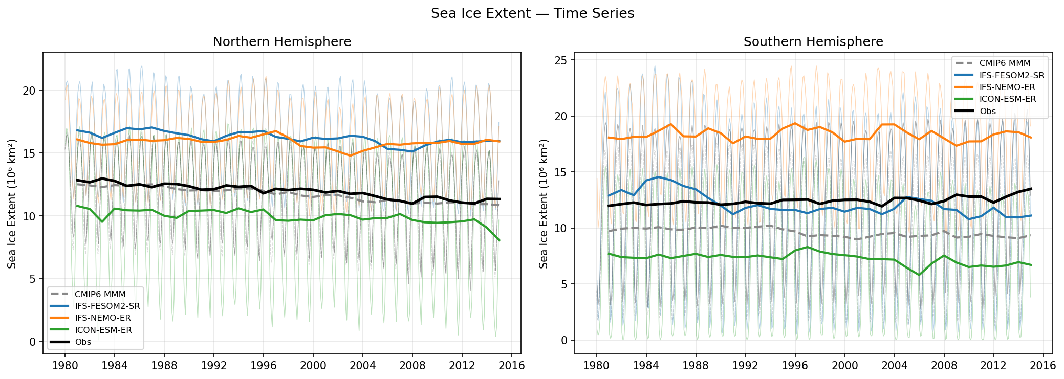
Summary high
This time series analysis evaluates monthly and annual-mean sea ice extent in the Northern (NH) and Southern Hemispheres (SH) for four high-resolution models against OSI-SAF observations. While HadGEM3-GC5 accurately reproduces NH decline, the models diverge significantly in the SH, with biases ranging from massive overestimation (IFS-NEMO-ER) to severe underestimation (ICON-ESM-ER, HadGEM3-GC5).
Key Findings
- HadGEM3-GC5 demonstrates excellent skill in the NH, closely tracking observed extent magnitude (~12-13 million km²) and the declining trend.
- IFS-NEMO-ER exhibits a strong systematic positive bias globally, overestimating NH extent by ~3-4 million km² and SH extent by an extreme ~6-7 million km².
- ICON-ESM-ER consistently underestimates sea ice in both hemispheres, with NH extent dropping rapidly below 10 million km² and SH extent remaining ~4-5 million km² below observations.
- The SH sea ice spread is vast: models do not agree on the mean state, with IFS-NEMO-ER showing extensive ice cover (~18 million km²) while HadGEM3-GC5 and ICON-ESM-ER predict a significantly reduced cryosphere (~8 million km²) relative to observations (~12.5 million km²).
Spatial Patterns
In the NH, observations show a clear downward trend from 1980 to 2014. HadGEM3-GC5 captures this rate well, whereas IFS models show a flatter trend and higher mean state. In the SH, observations show a slight positive trend/stability. IFS-FESOM2-SR starts near observations but drifts downward; IFS-NEMO-ER maintains a high, stable bias; and ICON/HadGEM3 maintain low, stable biases. The seasonal cycle amplitude in the SH is exaggerated in the high-bias IFS-NEMO-ER simulation.
Model Agreement
Inter-model agreement is moderate in the NH but extremely poor in the SH. In the NH, IFS-FESOM2-SR and IFS-NEMO-ER cluster together (high bias), while HadGEM3-GC5 aligns with the CMIP6 MMM and observations. In the SH, the models span a range of ~11 million km² in annual mean extent, far exceeding the observational uncertainty. HadGEM3-GC5 and ICON-ESM-ER fall below the CMIP6 MMM in the SH.
Physical Interpretation
The contrast between IFS-NEMO-ER (massive SH excess) and IFS-FESOM2-SR (moderate SH bias) is striking, as both share the IFS atmospheric component. This isolates the ocean/sea-ice model formulation (NEMO vs FESOM) as the primary driver of the Antarctic discrepancy. The shared positive bias in the NH for both IFS runs suggests the atmospheric forcing (e.g., cold biases or cloud feedbacks) may be dominant there. The low SH bias in HadGEM3-GC5 and ICON-ESM-ER is a common coupled model feature, often linked to excessive heat accumulation in the Southern Ocean or issues with open-ocean convection.
Caveats
- The definition of sea ice extent (e.g., 15% concentration threshold) is assumed consistent but grid-geometry differences between models can affect integrated metrics.
- The analysis period ends in 2014, excluding the recent extreme lows in Antarctic sea ice.
Sea Ice Volume March & September Trends
| Variables | siconc, sithick |
|---|---|
| Models | MPI-ESM1-2-LR, ACCESS-ESM1-5, EC-Earth3, CNRM-CM6-1, CNRM-ESM2-1, INM-CM5-0, MRI-ESM2-0, IFS-FESOM2-SR, IFS-NEMO-ER, ICON-ESM-ER, HadGEM3-GC5 |
| Reference Dataset | PSC |
| Units | 0-1 |
| Period | 1980–2014 |
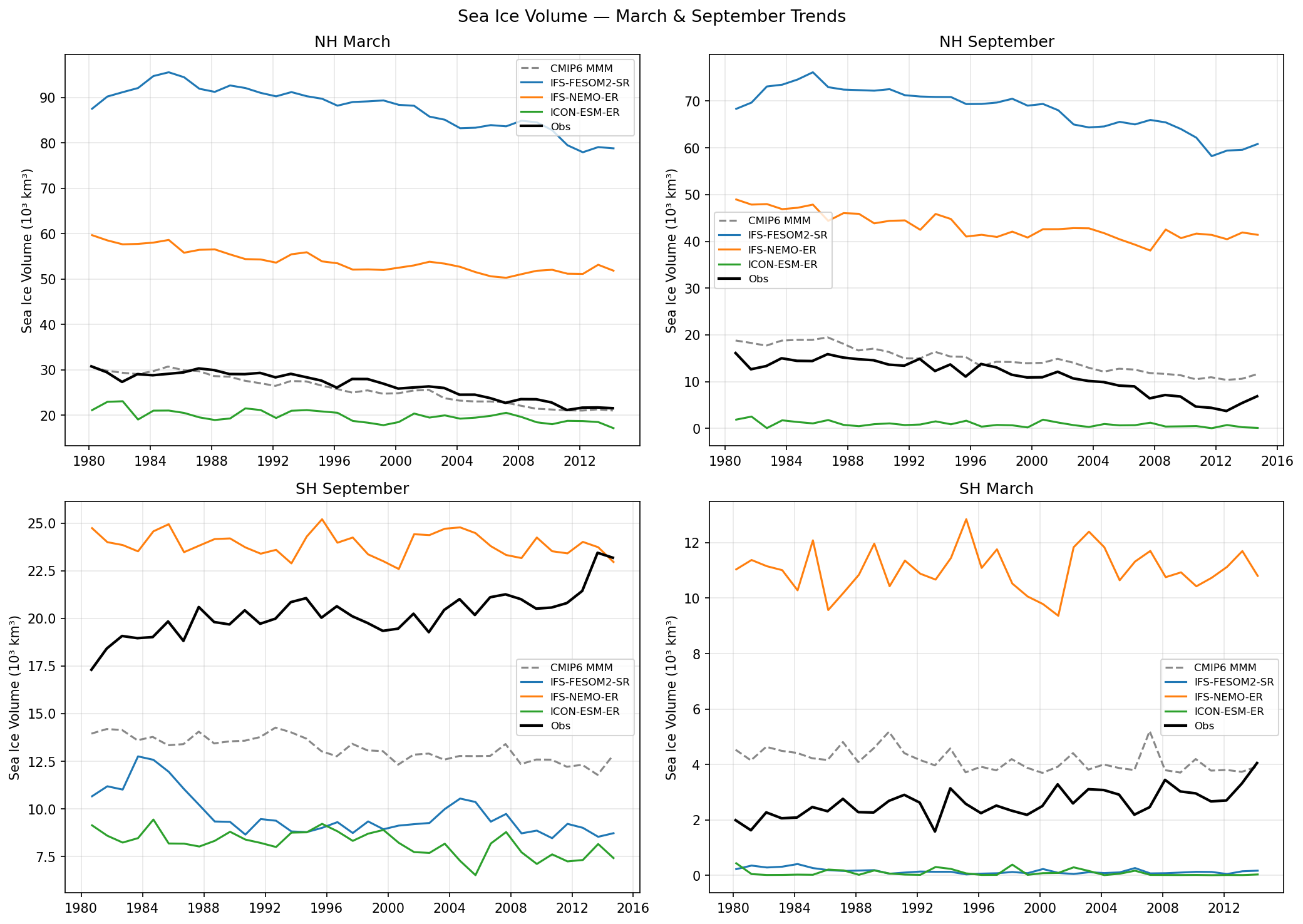
Summary high
This figure evaluates annual sea ice volume trends for March and September in the Northern and Southern Hemispheres (1980–2014) for four high-resolution models compared to PIOMAS reanalysis and CMIP6 context.
Key Findings
- IFS-FESOM2-SR exhibits an extreme positive bias in NH sea ice volume (~300% of observations), reaching ~90,000 km³ in March compared to ~30,000 km³ in PIOMAS.
- HadGEM3-GC5 performs best in the NH, closely tracking PIOMAS magnitudes and the precipitous decline in September volume.
- IFS-NEMO-ER consistently overestimates volume in both hemispheres, maintaining a positive bias throughout the period.
- ICON-ESM-ER consistently underestimates volume, predicting nearly ice-free NH summers (September volume <2,000 km³) throughout the historical period.
- In the SH, most models (HadGEM3, IFS-FESOM, ICON) underestimate volume compared to PIOMAS, while IFS-NEMO significantly overestimates it.
Spatial Patterns
The Northern Hemisphere shows a clear, multidecadal decline in volume across all datasets, most accurately captured by HadGEM3-GC5. The Southern Hemisphere observations show a slight positive trend or stability up to 2014, which the models struggle to reproduce, showing either flat or noisy trends with significant mean-state biases.
Model Agreement
There is very low inter-model agreement on mean state volume, with a spread exceeding the observational magnitude itself (e.g., NH March range of 20,000 to 90,000 km³). HadGEM3-GC5 is the only model that agrees well with the observational reference in the NH.
Physical Interpretation
Since sea ice area is spatially bounded, the massive volume biases (especially IFS-FESOM2-SR in NH and IFS-NEMO-ER globally) are driven by excessive ice thickness. This implies errors in thermodynamic growth/melt balances or dynamic piling-up of multi-year ice (insufficient export). Conversely, ICON-ESM-ER's low volume suggests excessive melting or insufficient formation, leading to thin first-year ice dominance. The SH discrepancies highlight the difficulty in simulating Antarctic sea ice processes (e.g., ocean stratification, wind-driven expansion) in coupled models.
Caveats
- PIOMAS is a reanalysis product (model constrained by observations), not direct observation, though it is the standard reference for volume.
- Southern Hemisphere volume data (often GIOMAS or similar) has higher uncertainty than NH.
Sea Ice Volume Seasonal Cycle
| Variables | siconc, sithick |
|---|---|
| Models | MPI-ESM1-2-LR, ACCESS-ESM1-5, EC-Earth3, CNRM-CM6-1, CNRM-ESM2-1, INM-CM5-0, MRI-ESM2-0, IFS-FESOM2-SR, IFS-NEMO-ER, ICON-ESM-ER, HadGEM3-GC5 |
| Reference Dataset | PSC |
| Units | 0-1 |
| Period | 1980–2014 |
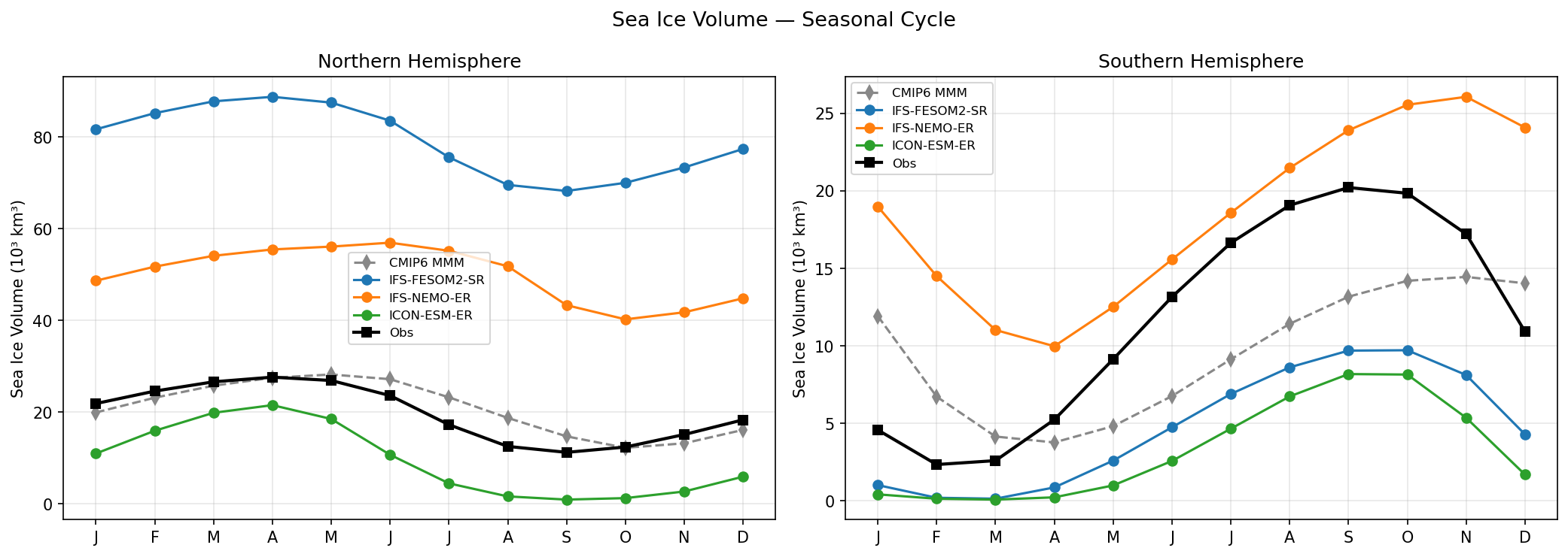
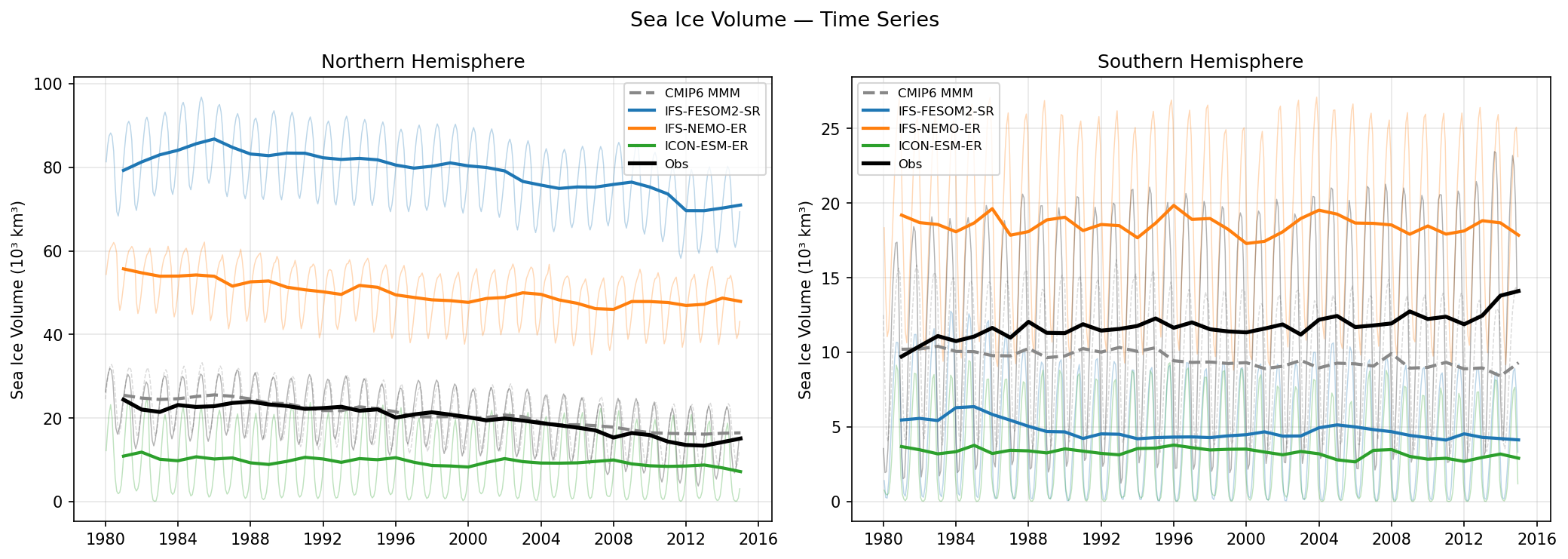
Summary high
This figure displays the seasonal cycle of Northern (NH) and Southern Hemisphere (SH) sea ice volume ($10^3$ km$^3$). It reveals massive inter-model discrepancies, with IFS-based models showing significant volume overestimations in the NH, while ICON-ESM-ER generally underestimates volume, particularly in the NH summer.
Key Findings
- IFS-FESOM2-SR exhibits an extreme positive bias in NH sea ice volume, ranging from 70–90 $10^3$ km$^3$, roughly 3–4 times the observational reference (~20–30 $10^3$ km$^3$).
- IFS-NEMO-ER also significantly overestimates NH volume (approx. double observations) and is the only model to overestimate SH volume, particularly during the austral summer minimum.
- ICON-ESM-ER generally underestimates sea ice volume; in the NH, it tracks observations in winter but melts nearly completely in summer (near-zero volume), while in the SH, it produces less than half the observed peak volume.
- The CMIP6 Multi-Model Mean (MMM) agrees reasonably well with observations in the NH, outperforming the high-resolution EERIE models, but underestimates peak volume in the SH.
Spatial Patterns
In the NH, the seasonal phase is generally captured by all models (max in Apr, min in Sept), but the mean state offsets are enormous. In the SH, IFS-NEMO-ER shows a distorted seasonal cycle with a very high summer minimum (~10 $10^3$ km$^3$ vs ~2.5 $10^3$ km$^3$ observed), suggesting excessive retention of multi-year ice.
Model Agreement
Inter-model agreement is very poor, with volume estimates differing by factors of 3-4. The high-resolution models generally deviate more from observations than the CMIP6 MMM ensemble average.
Physical Interpretation
The massive NH volume overestimates in IFS-FESOM2-SR and IFS-NEMO-ER imply excessive ice thickness, likely due to imbalances in thermodynamic growth/melt rates or albedo tuning, rather than just area biases. Conversely, ICON-ESM-ER's 'thin ice' bias (near-zero NH summer volume) suggests excessive surface melting or insufficient winter growth. The SH behavior of IFS-NEMO-ER suggests a failure to melt first-year ice during summer, leading to artificial multi-year ice accumulation.
Caveats
- Sea ice volume observations are typically derived from reanalyses (e.g., PIOMAS/GIOMAS) rather than direct satellite measurement, carrying higher uncertainty than concentration/extent data.
- The prompt metadata lists 'siconc' as the variable, but the plot clearly shows volume, implying thickness is integrated.
Sea Ice Volume Time Series
| Variables | siconc, sithick |
|---|---|
| Models | MPI-ESM1-2-LR, ACCESS-ESM1-5, EC-Earth3, CNRM-CM6-1, CNRM-ESM2-1, INM-CM5-0, MRI-ESM2-0, IFS-FESOM2-SR, IFS-NEMO-ER, ICON-ESM-ER, HadGEM3-GC5 |
| Reference Dataset | PSC |
| Units | 0-1 |
| Period | 1980–2014 |
Summary high
This figure evaluates monthly and annual-mean sea ice volume in the Northern (NH) and Southern (SH) Hemispheres from 1980–2014. There are massive discrepancies in mean state between models, with IFS-FESOM2-SR showing extreme ice volume overestimation in the NH, while HadGEM3-GC5 tracks the observational PIOMAS reanalysis most closely.
Key Findings
- In the NH, IFS-FESOM2-SR exhibits an extreme positive bias, simulating volumes (~80 × 10³ km³) nearly four times the PIOMAS observational reference (~20–25 × 10³ km³).
- HadGEM3-GC5 is the best-performing model for NH volume, capturing both the magnitude (~20–25 × 10³ km³) and the accelerating decline observed in PIOMAS, aligning well with the CMIP6 multi-model mean.
- In the SH, most models (HadGEM3-GC5, IFS-FESOM2-SR, ICON-ESM-ER) significantly underestimate sea ice volume (~5 × 10³ km³ vs ~12 × 10³ km³ in observations), whereas IFS-NEMO-ER overestimates it (~19 × 10³ km³).
- ICON-ESM-ER consistently underestimates sea ice volume in both hemispheres, producing the thinnest ice of all models evaluated.
Spatial Patterns
The NH time series shows a clear downward trend in the observational reference (PIOMAS) and HadGEM3-GC5, reflecting Arctic sea ice loss. The IFS variants show weaker relative trends due to their excessive mean states. In the SH, the observational reference shows a slight increase in volume over the period, a feature missed by the models, which generally show flat or slightly declining trends (consistent with the CMIP6 MMM failure to capture historical Antarctic sea ice expansion).
Model Agreement
Inter-model agreement is very poor regarding the mean state (total volume), with NH estimates ranging from ~10 × 10³ km³ (ICON) to ~80 × 10³ km³ (IFS-FESOM). However, the seasonal cycle phasing is generally consistent across models. Only HadGEM3-GC5 falls within the standard CMIP6 spread for the NH.
Physical Interpretation
The massive volume overestimation in IFS-FESOM2-SR (NH) and IFS-NEMO-ER (NH and SH) implies excessive ice thickness, likely driven by biases in thermodynamic growth (e.g., surface albedo tuning) or insufficient dynamical export. Conversely, ICON-ESM-ER's low volume suggests a warm bias in the polar oceans or atmosphere. The disconnect in the SH, where IFS-FESOM is low despite being high in the NH, suggests hemispherically distinct drivers, possibly related to Southern Ocean heat flux parameterizations or the representation of polynyas and stratification in the FESOM vs NEMO ocean components.
Caveats
- PIOMAS is a reanalysis product and is widely accepted for NH volume, but SH volume observations (labeled PIOMAS here, likely GIOMAS or similar proxy) have much higher uncertainty due to sparse thickness data.
- The extreme values in IFS-FESOM2-SR suggest a model drift or initialization issue that may distort other coupled feedbacks.
Arctic Sea Ice Concentration
| Variables | siconc |
|---|---|
| Models | IFS-FESOM2-SR, IFS-NEMO-ER, ICON-ESM-ER, HadGEM3-GC5 |
| Reference Dataset | OSI_SAF |
| Units | 0-1 |
| Period | 1980–2014 |
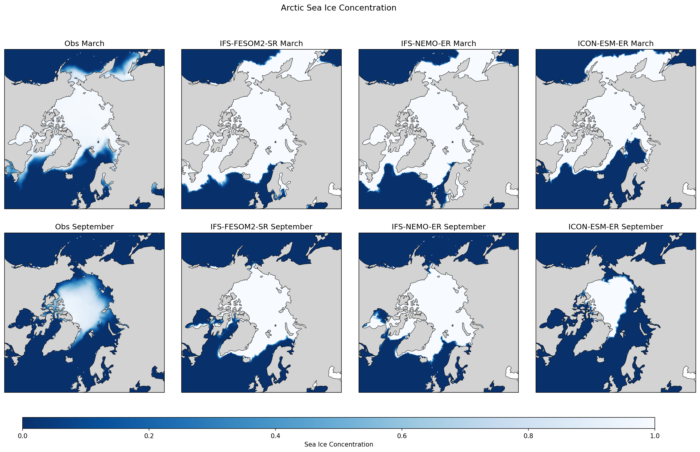
Summary high
This diagnostic compares Arctic sea ice concentration climatologies (March and September) from three high-resolution coupled models against OSI-SAF observations. IFS-FESOM2-SR demonstrates the best overall agreement with observations, while IFS-NEMO-ER and ICON-ESM-ER exhibit significant negative biases in specific seasons and regions.
Key Findings
- IFS-FESOM2-SR captures the spatial distribution of sea ice most accurately, reproducing both the winter extension into the Labrador Sea and the summer minimum extent well.
- IFS-NEMO-ER consistently underestimates sea ice concentration, with a retreated winter ice edge in the Barents/Labrador Seas and a severe underestimation of the September minimum, where the pack is significantly reduced and fragmented compared to observations.
- ICON-ESM-ER shows a strong 'warm winter' bias in the Atlantic sector, failing to form ice in the Labrador Sea and much of the Barents Sea in March, yet paradoxically maintains a robust, highly concentrated central ice pack in September.
Spatial Patterns
In March (winter maximum), the primary discrepancies are in the Atlantic marginal ice zones: observations show ice extending south to Newfoundland (Labrador Sea) and covering the Barents Sea. IFS-NEMO-ER and ICON-ESM-ER retreat the ice edge significantly northward in these regions. In September (summer minimum), models tend to show sharper gradients (binary 100% vs 0% concentration) compared to the diffuse marginal ice zone seen in observations. IFS-NEMO-ER exhibits a distinct 'hole' or severe thinning in the Eurasian sector of the Arctic basin in summer.
Model Agreement
Inter-model agreement is low, particularly in the marginal seas. IFS-FESOM2-SR aligns closely with observations, whereas IFS-NEMO-ER and ICON-ESM-ER diverge significantly from observations and each other, representing different failure modes (year-round underestimation vs. seasonal/regional contrast).
Physical Interpretation
The lack of winter ice in the Labrador and Barents Seas in IFS-NEMO-ER and ICON-ESM-ER suggests excessive oceanic heat transport from the North Atlantic (Atlantification) or warm atmospheric biases preventing ice formation. The severe summer melt in IFS-NEMO-ER indicates strong positive feedback loops (ice-albedo) or insufficient vertical stratification allowing sub-surface heat to erode the pack. The sharp concentration gradients in models compared to observations likely reflect both model parameterization of sub-grid ice thickness and the difficulty of satellite retrievals in distinguishing melt ponds from open water.
Caveats
- Satellite observations in September may underestimate ice concentration due to melt ponds on the ice surface being interpreted as open water.
- The 0-1 scale masks differences in ice thickness; a model could have 100% concentration but very thin ice.
Antarctic Sea Ice Concentration
| Variables | siconc |
|---|---|
| Models | IFS-FESOM2-SR, IFS-NEMO-ER, ICON-ESM-ER, HadGEM3-GC5 |
| Reference Dataset | OSI_SAF |
| Units | 0-1 |
| Period | 1980–2014 |
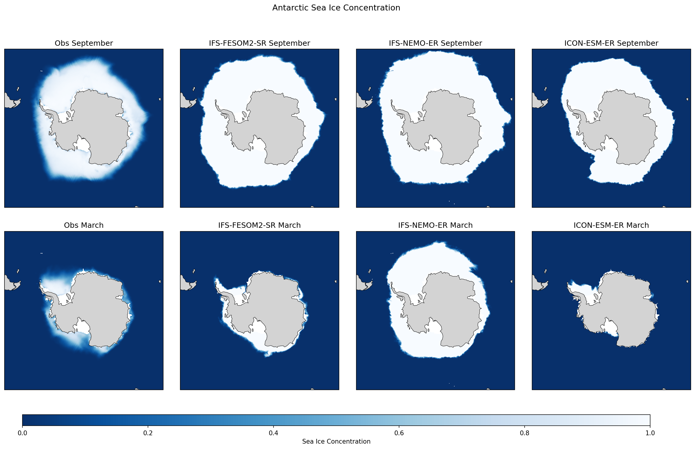
Summary high
This figure compares climatological Antarctic sea ice concentration for the annual maximum (September) and minimum (March) between four high-resolution coupled models and OSI-SAF observations. While models generally capture the broad spatial extent of the winter maximum, they diverge dramatically in the summer minimum, revealing severe opposing biases.
Key Findings
- Severe divergence in summer (March) sea ice: IFS-NEMO-ER retains an unrealistic, massive ice cover in the Weddell Sea sector, whereas IFS-FESOM2-SR, ICON-ESM-ER, and HadGEM3-GC5 nearly lose the entire ice pack, significantly underestimating the observed perennial ice.
- Winter (September) consistency: All models reproduce the circum-Antarctic ice extent reasonably well, though ICON-ESM-ER shows a slightly retracted ice edge in the Indian Ocean and Amundsen Sea sectors compared to observations.
- Weddell Sea biases: This region shows the largest model disagreement. IFS-NEMO-ER simulates a near-permanent ice shelf-like extension, while the other three models fail to maintain the observed perennial ice gyre.
Spatial Patterns
In September, observations show a continuous high-concentration ring; IFS-NEMO-ER produces the most extensive cover, while ICON-ESM-ER is the most limited. In March, observations show remnant ice in the Weddell Gyre and Amundsen/Ross sectors. IFS-NEMO-ER fills the Weddell sector with high-concentration ice (excessive), while IFS-FESOM2-SR, ICON-ESM-ER, and HadGEM3-GC5 show only thin coastal strips (deficient).
Model Agreement
Models agree on the general winter pattern but disagree fundamentally on summer dynamics. IFS-FESOM2-SR, ICON-ESM-ER, and HadGEM3-GC5 cluster together with a 'summer melt' bias, while IFS-NEMO-ER stands alone with a 'lack of melt' bias.
Physical Interpretation
The 'too little summer ice' bias in IFS-FESOM2, ICON, and HadGEM3 is a common coupled model issue, likely driven by warm biases in the Southern Ocean, excessive ocean heat uptake, or insufficient winter ice thickness (ice-albedo feedback). The extreme positive bias in IFS-NEMO-ER suggests a cold bias or issues with vertical mixing; if Warm Deep Water is not mixed upward effectively in the Weddell Gyre, the surface layer remains too fresh and cold, preventing summer melt and leading to unrealistic multi-year ice accumulation.
Caveats
- The figure shows climatology, masking interannual variability or trends (e.g., recent observed lows).
- Ice thickness is not shown but is crucial for diagnosing why the ice disappears or persists.
Arctic Sea Ice Thickness (m)
| Variables | sithick |
|---|---|
| Models | IFS-FESOM2-SR, IFS-NEMO-ER, ICON-ESM-ER, HadGEM3-GC5 |
| Reference Dataset | PSC |
| Units | m |
| Period | 1980–2014 |
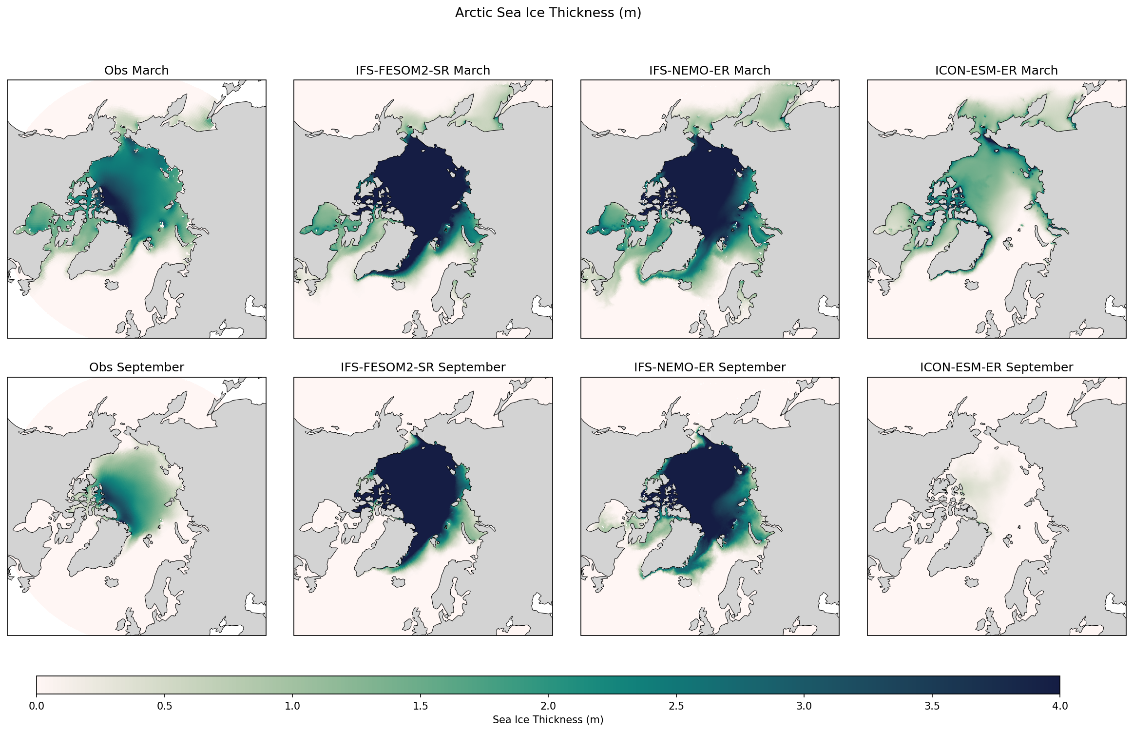
Summary high
This figure evaluates Arctic sea ice thickness in March (annual maximum) and September (annual minimum) for three high-resolution models against observations (likely PIOMAS reanalysis). The models exhibit starkly contrasting biases: both IFS-based models significantly overestimate ice thickness, while ICON-ESM-ER significantly underestimates it.
Key Findings
- IFS-FESOM2-SR and IFS-NEMO-ER exhibit a strong positive thickness bias, simulating widespread central Arctic ice exceeding 3.5–4.0 m in March, whereas observations show such thickness is confined to the region north of the Canadian Archipelago.
- ICON-ESM-ER exhibits a severe negative thickness bias, with March thickness rarely exceeding 2.0 m in the central basin and a near-total loss of sea ice in September (almost ice-free conditions).
- Both IFS models retain excessive thick ice (>3.0 m) throughout the summer (September), showing limited seasonal sensitivity compared to the observed retreat.
- The spatial gradient of thickness (thickest near Canadian/Greenland coast, thinning towards Siberia) is poorly represented in all models; IFS models show a 'homogenized' thick central basin, while ICON is uniformly thin.
Spatial Patterns
Observations show a characteristic wedge of thick multi-year ice (>3 m) north of Greenland and the Canadian Archipelago, thinning towards the Siberian coast. IFS-FESOM2-SR and IFS-NEMO-ER extend this thick zone across the entire central Arctic basin, creating a massive area of ice >3.5 m. Conversely, ICON-ESM-ER fails to maintain this thick reservoir even in March, leading to a thin, fragile ice pack that largely vanishes in September.
Model Agreement
There is very low inter-model agreement. The models bifurcate into two extremes: the IFS-driven models (using FESOM and NEMO oceans) are 'too cold/thick', while the ICON model is 'too warm/thin'. None of the models closely reproduce the observational magnitude of sea ice thickness, though the IFS models capture the March spatial extent boundaries better than ICON captures the September extent.
Physical Interpretation
The excessive thickness in IFS-FESOM2 and IFS-NEMO suggests either insufficient summer melting (albedo feedback, cloud radiative forcing) or excessive thermodynamic growth/dynamic convergence. The similarity between the two IFS variants implies the atmospheric driver (IFS) or common tuning may dominate over ocean model differences (FESOM vs. NEMO). The thinning in ICON-ESM-ER suggests overly efficient ocean heat transport to the surface, insufficient insulation, or biases in surface energy balance leading to rapid melt. The lack of thick multi-year ice in ICON indicates the model fails to survive the melt season to build up thickness over years.
Caveats
- The 'Obs' dataset is not specified but is likely a reanalysis product like PIOMAS, as direct satellite thickness observations (e.g., CryoSat-2) are limited for the 1980–2014 period.
- Averaging over 1980–2014 masks the strong observed trend of thinning ice; however, the model biases are large enough to be distinct from trend-related errors.
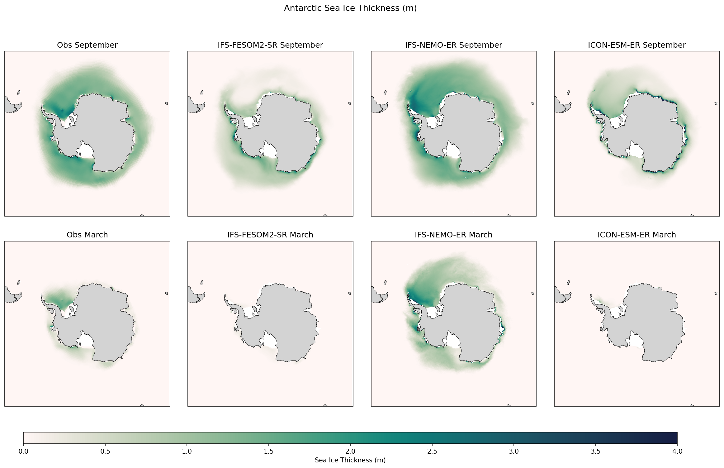
Antarctic Sea Ice Thickness (m)
| Variables | sithick |
|---|---|
| Models | IFS-FESOM2-SR, IFS-NEMO-ER, ICON-ESM-ER, HadGEM3-GC5 |
| Reference Dataset | PSC |
| Units | m |
| Period | 1980–2014 |
Summary medium
This figure evaluates Antarctic sea ice thickness and seasonal evolution (September maximum vs. March minimum) in four high-resolution coupled models against PIOMAS reanalysis. The models exhibit large divergences in mean state, ranging from severe thinning/summer loss to excessive thickening.
Key Findings
- IFS-NEMO-ER shows a strong positive bias, simulating excessive ice thickness (>2.5 m) in the Weddell and Amundsen Seas in September and retaining unrealistic widespread ice cover in March.
- IFS-FESOM2-SR and ICON-ESM-ER exhibit severe negative biases in summer (March), producing nearly ice-free conditions and failing to capture the observed survival of multi-year ice in the Weddell Sea.
- ICON-ESM-ER produces generally thin ice (<1 m) across most of the Antarctic pack even in winter (September), suggesting insufficient thermodynamic growth or excessive ocean heat flux.
- HadGEM3-GC5 shows the best agreement with PIOMAS, capturing the spatial structure of thicker ice in the Weddell Sea and maintaining a realistic extent of remnant ice in March.
Spatial Patterns
In PIOMAS, the thickest ice (>2 m) is concentrated in the Weddell Sea and along the Antarctic Peninsula. IFS-NEMO-ER exaggerates this feature with a vast area of thick ice. Conversely, IFS-FESOM2-SR and ICON-ESM-ER lack this structural accumulation, leading to their inability to sustain ice through the summer melt season.
Model Agreement
Inter-model agreement is poor. The models span the full range from too thin (ICON) to too thick (IFS-NEMO), with only HadGEM3-GC5 reasonably approximating the reanalysis. Notably, IFS-NEMO and IFS-FESOM share the same atmospheric component but show opposite biases, isolating the ocean/sea-ice formulation as the primary driver.
Physical Interpretation
The excessive thickness in IFS-NEMO-ER suggests issues with ice rheology (piling up too easily) or insufficient basal melt/export. The thinness in ICON-ESM-ER and IFS-FESOM2-SR implies either excessive summer shortwave absorption (albedo feedback), insufficient winter growth, or too much vertical mixing bringing warm deep water to the surface (common in Southern Ocean models). The specific failure to maintain Weddell Sea multi-year ice in two models points to dynamic deficiencies in the Weddell Gyre circulation or thermodynamic biases.
Caveats
- PIOMAS is a reanalysis (model constrained by observations), not direct observation. Antarctic sea ice thickness observations are sparse, so PIOMAS has higher uncertainty here than in the Arctic.
- The label 'PIOMAS' usually refers to an Arctic reanalysis; this is likely a global or Antarctic-specific variant (e.g., GIOMAS), which may have its own biases.