Evaluation Climate Variability (ERA5) CMIP6
CMIP6 Multi-Model Mean Context
Comparison with CMIP6 ensemble mean from 11 members.
Contributing models: ACCESS-ESM1-5, AWI-CM-1-1-MR, CNRM-CM6-1, CNRM-ESM2-1, EC-Earth3, FGOALS-g3, GISS-E2-1-G, INM-CM5-0, IPSL-CM6A-LR, MPI-ESM1-2-LR, MRI-ESM2-0
Synthesis
Related diagnostics
Total Cloud Cover — Variability (STD)
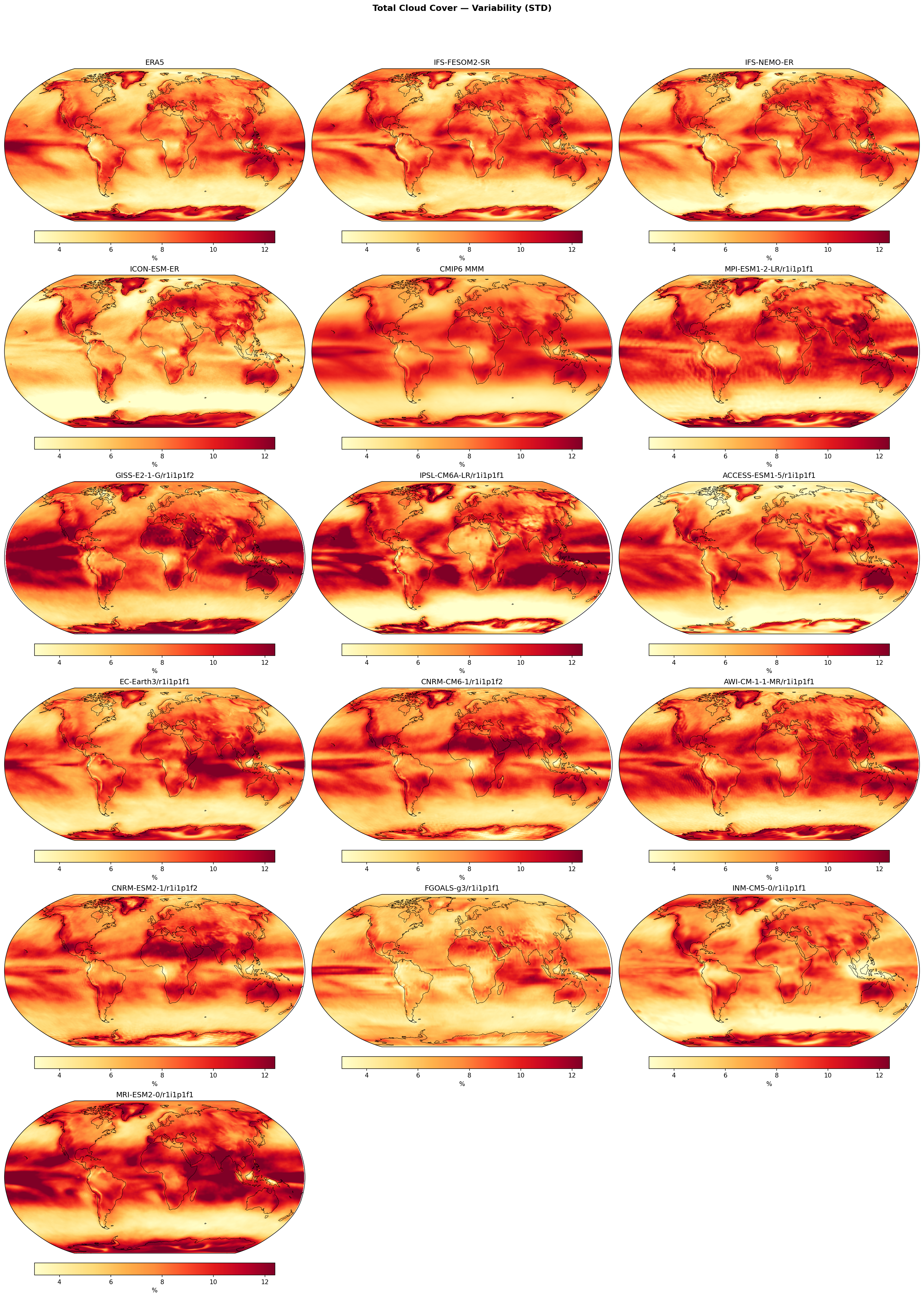
| Variables | clt |
|---|---|
| Models | IFS-FESOM2-SR, IFS-NEMO-ER, ICON-ESM-ER, HadGEM3-GC5, CMIP6 MMM, MPI-ESM1-2-LR/r1i1p1f1, GISS-E2-1-G/r1i1p1f2, IPSL-CM6A-LR/r1i1p1f1, ACCESS-ESM1-5/r1i1p1f1, EC-Earth3/r1i1p1f1, CNRM-CM6-1/r1i1p1f2, AWI-CM-1-1-MR/r1i1p1f1, CNRM-ESM2-1/r1i1p1f2, FGOALS-g3/r1i1p1f1, INM-CM5-0/r1i1p1f1, MRI-ESM2-0/r1i1p1f1 |
| Reference Dataset | ERA5 |
| Units | % |
| Period | 1980–2014 |
| IFS-FESOM2-SR | Std Gmean: 7.59 · Diff Gmean: 0.24 · Rmse: 1.21 |
| IFS-NEMO-ER | Std Gmean: 7.39 · Diff Gmean: 0.04 · Rmse: 1.00 |
| ICON-ESM-ER | Std Gmean: 6.38 · Diff Gmean: -0.96 · Rmse: 2.03 |
| HadGEM3-GC5 | Std Gmean: 6.28 · Diff Gmean: -1.07 · Rmse: 1.66 |
| CMIP6 MMM | Std Gmean: 8.13 · Diff Gmean: 0.78 · Rmse: 1.28 |
Summary high
This figure evaluates the temporal variability of total cloud cover (1980–2014) by comparing the standard deviation of deseasonalised, detrended monthly anomalies in EERIE models, CMIP6, and ERA5. IFS-based models exhibit excellent agreement with observations, whereas ICON and HadGEM3 systematic underestimate variability, and CMIP6 models generally overestimate it.
Key Findings
- IFS-NEMO-ER demonstrates the best performance with a global mean variability (7.39%) almost identical to ERA5 (~7.35%) and the lowest RMSE (1.00%).
- ICON-ESM-ER and HadGEM3-GC5 significantly underestimate cloud variability globally (biases of -0.96% and -1.07% respectively), appearing visually muted in storm tracks and the tropics.
- CMIP6 models (MMM and individuals like GISS-E2-1-G, IPSL-CM6A-LR) tend to overestimate cloud variability (MMM bias +0.78%), showing much higher amplitudes in the tropics and mid-latitudes than ERA5.
- The spatial signature of ENSO in the tropical Pacific is well-captured by ERA5 and IFS models but appears weaker and less coherent in ICON-ESM-ER.
Spatial Patterns
Highest cloud variability (>10-12%) is observed in the mid-latitude storm tracks (North Atlantic, North Pacific, Southern Ocean) and the tropical Pacific (ENSO tongue). Low variability characterizes the subtropical subsidence regions. IFS models reproduce these high-variability bands with accurate intensity and location. In contrast, ICON and HadGEM3 show reduced variability in the Southern Ocean storm track and a less distinct ENSO signature. CMIP6 models often show excessive variability over the tropical oceans.
Model Agreement
There is a distinct divergence in model behavior: IFS models align closely with ERA5 (RMSE ~1.0-1.2%), while ICON and HadGEM3 form a 'low variability' cluster (RMSE ~1.6-2.0%), and the broader CMIP6 ensemble forms a 'high variability' cluster. The IFS-NEMO-ER simulation is nearly indistinguishable from ERA5 in terms of global mean statistics and spatial patterns.
Physical Interpretation
The standard deviation of monthly cloud cover reflects the model's simulation of synoptic activity (storm tracks) and interannual modes (ENSO). The close match of IFS suggests its atmospheric physics and resolution successfully capture the frequency and amplitude of frontal passages and convective organization. The underestimation in ICON and HadGEM3 suggests either overly persistent cloud regimes (damped response to dynamical forcing) or dampened internal climate variability. Conversely, the high variability in many CMIP6 models implies overly sensitive cloud radiative responses or excessive dynamical variance.
Caveats
- The analysis relies on ERA5 reanalysis as truth; while robust, satellite-based climatologies (e.g., CLARA-A2) could provide an alternative observational perspective.
- The metric combines synoptic and interannual variability; separating these timescales could clarify if the bias stems from weather noise or climate modes like ENSO.
Total Cloud Cover — Variability Bias (STD diff)
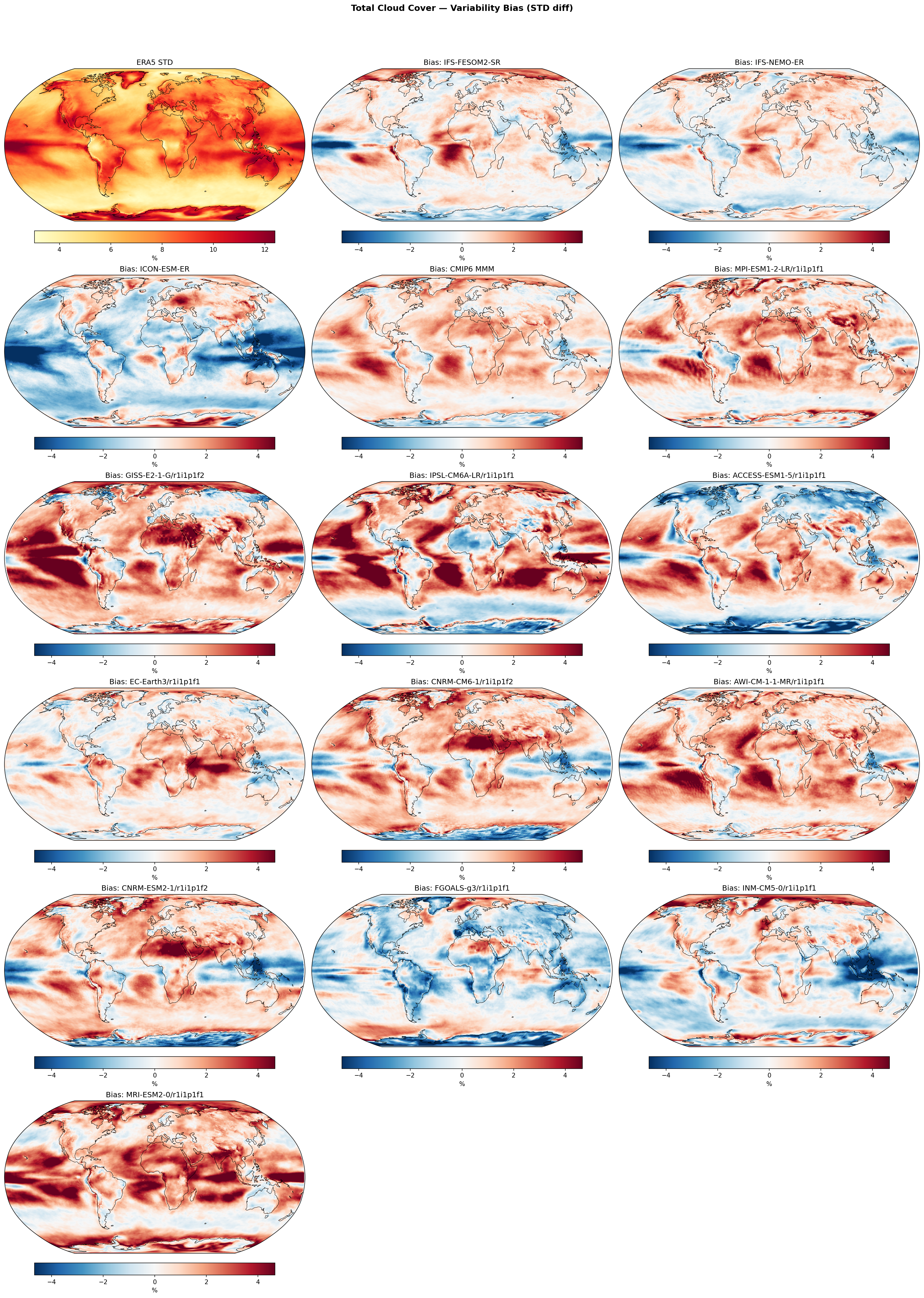
| Variables | clt |
|---|---|
| Models | IFS-FESOM2-SR, IFS-NEMO-ER, ICON-ESM-ER, HadGEM3-GC5, CMIP6 MMM, MPI-ESM1-2-LR/r1i1p1f1, GISS-E2-1-G/r1i1p1f2, IPSL-CM6A-LR/r1i1p1f1, ACCESS-ESM1-5/r1i1p1f1, EC-Earth3/r1i1p1f1, CNRM-CM6-1/r1i1p1f2, AWI-CM-1-1-MR/r1i1p1f1, CNRM-ESM2-1/r1i1p1f2, FGOALS-g3/r1i1p1f1, INM-CM5-0/r1i1p1f1, MRI-ESM2-0/r1i1p1f1 |
| Reference Dataset | ERA5 |
| Units | % |
| Period | 1980–2014 |
| IFS-FESOM2-SR | Std Gmean: 7.59 · Diff Gmean: 0.24 · Rmse: 1.21 |
| IFS-NEMO-ER | Std Gmean: 7.39 · Diff Gmean: 0.04 · Rmse: 1.00 |
| ICON-ESM-ER | Std Gmean: 6.38 · Diff Gmean: -0.96 · Rmse: 2.03 |
| HadGEM3-GC5 | Std Gmean: 6.28 · Diff Gmean: -1.07 · Rmse: 1.66 |
| CMIP6 MMM | Std Gmean: 8.13 · Diff Gmean: 0.78 · Rmse: 1.28 |
Summary high
This figure evaluates the variability (standard deviation) of Total Cloud Cover (TCC) in EERIE high-resolution simulations and CMIP6 models against ERA5 reanalysis. IFS-NEMO-ER demonstrates exceptional skill in reproducing observed variability patterns, while ICON-ESM-ER and HadGEM3-GC5 significantly underestimate variability globally, and the CMIP6 Multi-Model Mean generally overestimates it.
Key Findings
- IFS-NEMO-ER shows the lowest global biases (RMSE ~1.00%, mean bias ~0.04%), closely matching ERA5 variability magnitude and spatial structure.
- ICON-ESM-ER and HadGEM3-GC5 exhibit widespread negative biases (blue), indicating they underestimate cloud cover variability by ~1% in the global mean, particularly over the oceans.
- The CMIP6 Multi-Model Mean and several individual CMIP6 models (e.g., GISS-E2-1-G, IPSL-CM6A-LR) show strong positive biases (red) in the tropics, overestimating variability by >4% in convective regions.
- Common regional biases include underestimated variability in eastern boundary upwelling zones (stratocumulus decks) across multiple models, including IFS-FESOM2-SR and CMIP6 MMM.
Spatial Patterns
ERA5 shows peak cloud variability (8-12%) in the ITCZ/SPCZ and mid-latitude storm tracks. Biases are spatially coherent: positive biases are concentrated in the tropical convective zones (especially Pacific and Indian Oceans) for IFS-FESOM2-SR and CMIP6 models. Negative biases dominate the extratropical oceans and stratocumulus regions for ICON-ESM-ER and HadGEM3-GC5. The stratocumulus regions (e.g., off Peru, Namibia) show negative variability biases in most models, suggesting persistent cloud decks or persistent clear sky without the observed dynamic transitions.
Model Agreement
There is a distinct divergence between the IFS family and the ICON/HadGEM3 models. IFS-NEMO-ER aligns well with ERA5, while ICON and HadGEM3 systematic underestimate variability. The CMIP6 ensemble shows large inter-model spread, with end-members like GISS-E2-1-G (extreme positive bias) and FGOALS-g3 (extreme negative bias), though the ensemble mean leans towards overestimation.
Physical Interpretation
The positive variability bias in the tropics (seen in IFS-FESOM2-SR and CMIP6) likely stems from convective parameterizations triggering precipitation and cloud formation too intermittently ('popcorn convection'), leading to excessive fluctuation compared to reality. Conversely, the negative bias in ICON-ESM-ER and HadGEM3-GC5 suggests cloud schemes that produce too-persistent cloud cover or dampen synoptic variability. The widespread negative bias in stratocumulus regions implies models struggle to capture the specific synoptic-scale variability of these boundary layer clouds.
Caveats
- ERA5 cloud cover is a model-derived product (reanalysis) rather than direct satellite observation, though it assimilates relevant radiances.
- Biases in variability do not indicate biases in mean cloud fraction; a model could have correct mean cloudiness but incorrect temporal dynamics.
Surface Latent Heat Flux — Variability (STD)
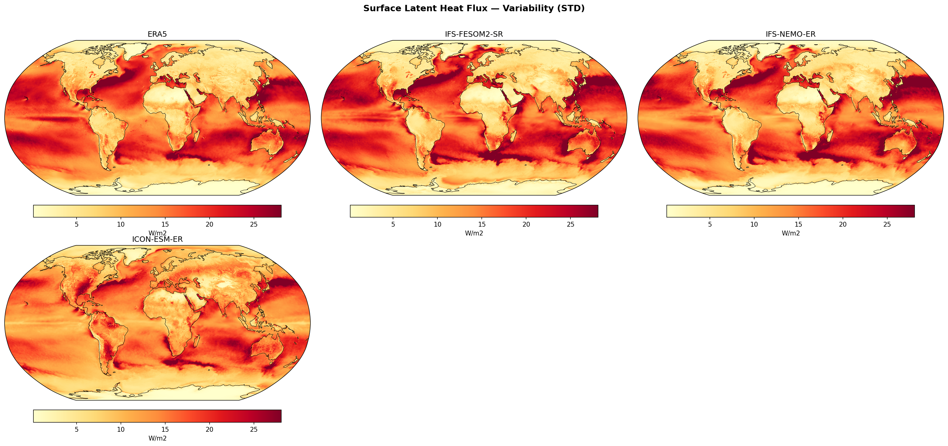
| Variables | hfls |
|---|---|
| Models | IFS-FESOM2-SR, IFS-NEMO-ER, ICON-ESM-ER |
| Reference Dataset | ERA5 |
| Units | W/m2 |
| Period | 1980–2014 |
| IFS-FESOM2-SR | Std Gmean: 14.69 · Diff Gmean: 0.80 · Rmse: 3.34 |
| IFS-NEMO-ER | Std Gmean: 14.02 · Diff Gmean: 0.12 · Rmse: 2.94 |
| ICON-ESM-ER | Std Gmean: 13.14 · Diff Gmean: -0.75 · Rmse: 5.09 |
Summary high
This diagnostic assesses the variability (standard deviation) of deseasonalised surface latent heat flux, highlighting regions of strong ocean-atmosphere interaction such as western boundary currents and storm tracks.
Key Findings
- All high-resolution models successfully capture the intense variability (>25 W/m²) associated with Western Boundary Currents (Gulf Stream, Kuroshio) and the Southern Ocean storm track, consistent with ERA5.
- IFS-NEMO-ER demonstrates the best performance with the lowest RMSE (2.94 W/m²) and a global mean difference closest to zero, reproducing ERA5 patterns with high fidelity.
- ICON-ESM-ER exhibits distinct biases: it significantly overestimates variability over tropical land masses (Amazon, Central Africa) while appearing to underestimate variability in the tropical Pacific and subtropical oceans compared to the IFS models and ERA5.
Spatial Patterns
Variability is maximised in Western Boundary Currents, the Agulhas Return Current, and major storm tracks due to synoptic activity and ocean fronts. A secondary maximum exists in the tropical Pacific (ENSO signature), while subtropical gyres remain quiescent.
Model Agreement
The two IFS-based models (NEMO and FESOM2) show strong agreement with ERA5 and each other. ICON-ESM-ER diverges significantly, particularly in its land-sea contrast, showing excessive volatility in terrestrial latent heat fluxes.
Physical Interpretation
Oceanic variability is driven by SST anomalies (eddies, fronts) and wind variability acting on moisture gradients. The high variability in WBCs confirms the models' eddy-rich nature enhances air-sea coupling. ICON's excessive land variability suggests issues in the land surface model's coupling strength (soil moisture-evaporation feedback) or forcing precipitation variability.
Caveats
- ICON-ESM-ER's negative global mean bias (-0.75 W/m²) is a net result of widespread weak ocean variability offsetting intense localised land variability.
- The analysis relies on ERA5 as truth, which itself is a model-derived reanalysis product.
Surface Latent Heat Flux — Variability Bias (STD diff)
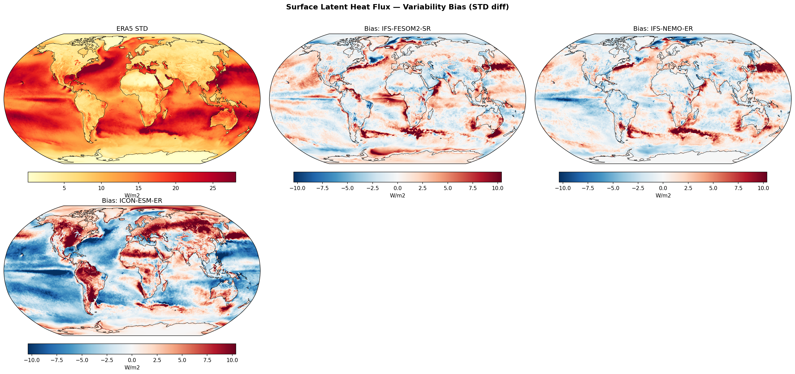
| Variables | hfls |
|---|---|
| Models | IFS-FESOM2-SR, IFS-NEMO-ER, ICON-ESM-ER |
| Reference Dataset | ERA5 |
| Units | W/m2 |
| Period | 1980–2014 |
| IFS-FESOM2-SR | Std Gmean: 14.69 · Diff Gmean: 0.80 · Rmse: 3.34 |
| IFS-NEMO-ER | Std Gmean: 14.02 · Diff Gmean: 0.12 · Rmse: 2.94 |
| ICON-ESM-ER | Std Gmean: 13.14 · Diff Gmean: -0.75 · Rmse: 5.09 |
Summary high
This diagnostic assesses the variability (standard deviation) of surface latent heat flux in three high-resolution coupled models compared to ERA5 reanalysis. The IFS-based models exhibit similar bias structures with excessive variability in western boundary currents, whereas ICON-ESM-ER shows a distinct contrast of suppressed oceanic variability and excessive land surface variability.
Key Findings
- IFS-NEMO-ER and IFS-FESOM2-SR show strong positive variability biases (>5-10 W/m²) in Western Boundary Currents (Gulf Stream, Kuroshio, Agulhas), indicating overly energetic air-sea interactions in these eddy-rich regions.
- ICON-ESM-ER displays a stark land-ocean contrast: it strongly overestimates latent heat flux variability over Northern Hemisphere continents and tropical rainforests, while underestimating it across most ocean basins, particularly in the Gulf Stream and Kuroshio extensions.
- IFS-NEMO-ER achieves the best overall agreement with ERA5 (RMSE ~2.94 W/m²), closely followed by IFS-FESOM2-SR, while ICON-ESM-ER has significantly higher errors (RMSE ~5.09 W/m²).
Spatial Patterns
ERA5 shows peak variability (>25 W/m²) in western boundary currents and tropical oceans. Both IFS models exaggerate this variability in the boundary currents but underestimate it in the central equatorial Pacific (cold tongue) and ITCZ regions. ICON-ESM-ER is characterized by widespread negative biases over the oceans (damping of flux variance) and intense positive biases over land regions like North America, Eurasia, and the Amazon.
Model Agreement
The two IFS-based models (IFS-FESOM2-SR and IFS-NEMO-ER) show high agreement in their spatial bias patterns, suggesting the atmospheric model component (IFS) or its coupling strategy dominates the flux variability characteristics. ICON-ESM-ER diverges significantly, showing opposite signs of bias in key regions like the Western Boundary Currents.
Physical Interpretation
The positive biases in IFS models over western boundary currents suggest intense turbulent heat flux exchanges, possibly driven by resolved mesoscale ocean eddies or strong atmospheric response to SST gradients. The negative bias in the equatorial Pacific in all models may indicate issues with ENSO amplitude or the positioning of the ITCZ/cold tongue. ICON's excessive land variability likely points to deficiencies in its land surface model (e.g., soil moisture memory or evapotranspiration parameterization), while its oceanic damping implies sluggish surface wind or humidity responses.
Caveats
- ERA5 latent heat fluxes are derived from bulk formulae and model physics, not direct observations, which carries its own uncertainties.
- Differences in land-sea mask resolution may affect coastal comparisons.
Surface Sensible Heat Flux — Variability (STD)
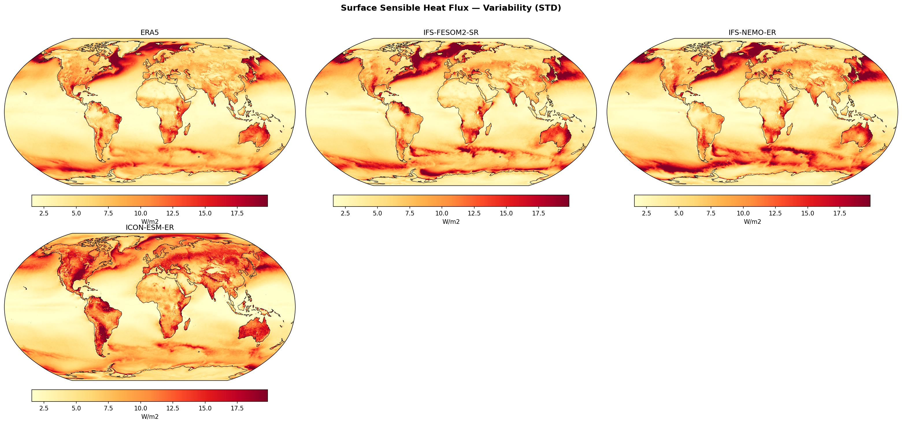
| Variables | hfss |
|---|---|
| Models | IFS-FESOM2-SR, IFS-NEMO-ER, ICON-ESM-ER |
| Reference Dataset | ERA5 |
| Units | W/m2 |
| Period | 1980–2014 |
| IFS-FESOM2-SR | Std Gmean: 6.45 · Diff Gmean: 0.49 · Rmse: 2.48 |
| IFS-NEMO-ER | Std Gmean: 6.57 · Diff Gmean: 0.61 · Rmse: 2.50 |
| ICON-ESM-ER | Std Gmean: 6.74 · Diff Gmean: 0.79 · Rmse: 3.43 |
Summary high
This figure displays the variability (standard deviation) of deseasonalised, detrended monthly Surface Sensible Heat Flux (SSHF) for three high-resolution models compared to ERA5 reanalysis. While oceanic patterns associated with boundary currents and sea ice are well-captured by all models, significant divergence occurs over land, particularly in ICON-ESM-ER.
Key Findings
- All models successfully reproduce the high SSHF variability hotspots over the Western Boundary Currents (Gulf Stream, Kuroshio) and the Southern Ocean marginal ice zones.
- IFS-FESOM2-SR and IFS-NEMO-ER show high skill, visually indistinguishable from each other and closely matching ERA5 patterns and magnitudes over both land and ocean (RMSE ~2.5 W/m²).
- ICON-ESM-ER systematically overestimates SSHF variability over major continental regions, specifically the Amazon basin, central Africa, and northern Eurasia, resulting in a higher global RMSE (~3.4 W/m²).
Spatial Patterns
Dominant variability features include the Western Boundary Currents (driven by strong air-sea temperature gradients during cold air outbreaks), the marginal ice zones (driven by sea ice retreat/advance exposing open water), and continental interiors (driven by synoptic weather systems). Tropical oceans exhibit notably low SSHF variability compared to high latitudes.
Model Agreement
The two IFS-based models (FESOM and NEMO) exhibit strong agreement with ERA5 and each other, indicating that the ocean grid discretization (finite element vs. finite difference) has minimal impact on surface flux variability at this resolution. ICON-ESM-ER is an outlier, agreeing well over the ocean but diverging significantly over land with excessive variability.
Physical Interpretation
Oceanic variability is physically driven by turbulent heat exchange in regions of high eddy activity and strong SST gradients (WBCs) and the drastic surface boundary condition changes at sea-ice edges. The excess variability in ICON over land suggests potential issues in the land-surface coupling (e.g., soil moisture-temperature feedbacks) or excessive surface temperature variance in the land model component.
Caveats
- The analysis uses monthly data, which filters out high-frequency synoptic variability that contributes significantly to sensible heat fluxes.
- ERA5 fluxes are derived from model parameterisations assimilating observational data, not direct observations, though they are considered a robust reference.
Surface Sensible Heat Flux — Variability Bias (STD diff)
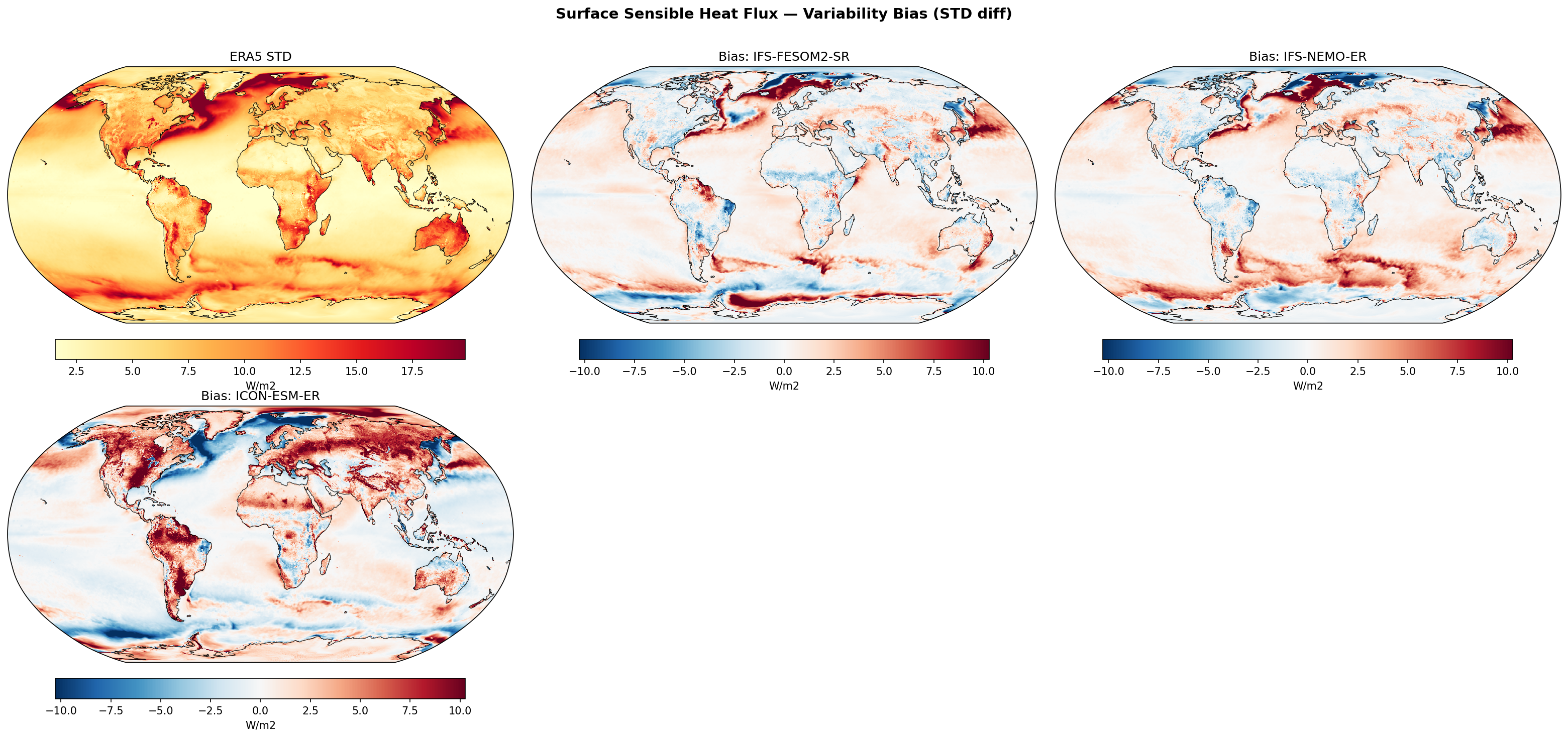
| Variables | hfss |
|---|---|
| Models | IFS-FESOM2-SR, IFS-NEMO-ER, ICON-ESM-ER |
| Reference Dataset | ERA5 |
| Units | W/m2 |
| Period | 1980–2014 |
| IFS-FESOM2-SR | Std Gmean: 6.45 · Diff Gmean: 0.49 · Rmse: 2.48 |
| IFS-NEMO-ER | Std Gmean: 6.57 · Diff Gmean: 0.61 · Rmse: 2.50 |
| ICON-ESM-ER | Std Gmean: 6.74 · Diff Gmean: 0.79 · Rmse: 3.43 |
Summary high
This diagnostic evaluates the variability (standard deviation) of Surface Sensible Heat Flux (SSHF) in three high-resolution coupled models compared to ERA5. The IFS-based models perform similarly with moderate biases focused in ocean frontal zones, while ICON-ESM-ER exhibits significantly higher widespread variability bias, particularly over land.
Key Findings
- All models overestimate SSHF variability in Western Boundary Currents (Gulf Stream, Kuroshio) relative to ERA5, likely reflecting sharper SST fronts and more energetic air-sea interaction at high resolution.
- ICON-ESM-ER displays a distinct, widespread positive variability bias over Northern Hemisphere land masses and tropical South America/Africa, contributing to a higher global RMSE (3.43 W/m²) compared to IFS models (~2.5 W/m²).
- Southern Ocean biases diverge significantly: IFS models show a band of excessive variability (positive bias) around 40-50°S, while ICON shows a strong negative bias band near the Antarctic coast, indicative of differing sea ice edge dynamics and open-ocean convection.
Spatial Patterns
ERA5 shows peak variability (>17 W/m²) in boundary currents and sea ice margins. Models reproduce these hotspots but amplify the magnitude in the Gulf Stream and Kuroshio extensions (red bias). Over land, IFS models are relatively neutral with patchy biases, whereas ICON is systematically 'red' (excessive variability) over most continents. High-latitude oceans show dipole bias patterns associated with sea ice margin mismatches.
Model Agreement
IFS-FESOM2-SR and IFS-NEMO-ER show high spatial agreement, confirming that the atmospheric component (IFS) dominates the surface flux characteristics. ICON-ESM-ER is an outlier with much stronger land biases and distinct polar ocean patterns.
Physical Interpretation
The positive bias in boundary currents may represent 'added value' where high-resolution models resolve sharper mesoscale eddies and fronts than the coarser ERA5 reanalysis. ICON's excessive land variability suggests a land-surface scheme issue, possibly related to soil moisture-limited evaporation regimes shifting energy partitioning erratically to sensible heat. The sea ice margin biases (dipoles) result from differences in the mean position and variance of the sea ice edge, which acts as a strong insulator/conductor switch for heat flux.
Caveats
- ERA5 surface fluxes are derived from bulk formulae and model physics, not directly observed, so 'bias' in highly active regions might reflect reanalysis limitations.
- Higher variability in eddy-rich regions in high-res models is physically expected and may not strictly constitute an error.
Total Precipitation Rate — Variability (STD)
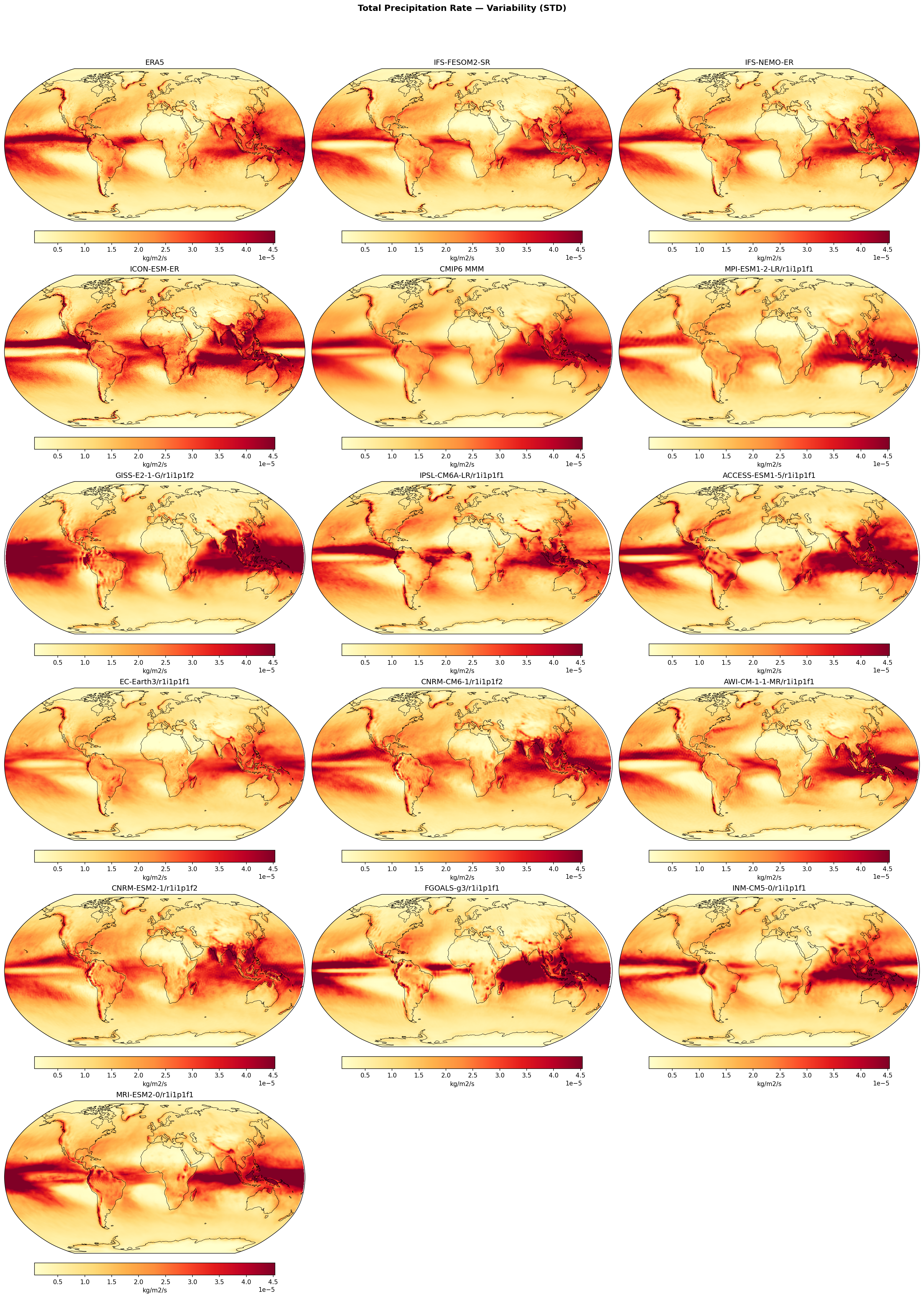
| Variables | pr |
|---|---|
| Models | IFS-FESOM2-SR, IFS-NEMO-ER, ICON-ESM-ER, HadGEM3-GC5, CMIP6 MMM, MPI-ESM1-2-LR/r1i1p1f1, GISS-E2-1-G/r1i1p1f2, IPSL-CM6A-LR/r1i1p1f1, ACCESS-ESM1-5/r1i1p1f1, EC-Earth3/r1i1p1f1, CNRM-CM6-1/r1i1p1f2, AWI-CM-1-1-MR/r1i1p1f1, CNRM-ESM2-1/r1i1p1f2, FGOALS-g3/r1i1p1f1, INM-CM5-0/r1i1p1f1, MRI-ESM2-0/r1i1p1f1 |
| Reference Dataset | ERA5 |
| Units | kg/m2/s |
| Period | 1980–2014 |
| IFS-FESOM2-SR | Std Gmean: 0.00 · Diff Gmean: 0.00 · Rmse: 0.00 |
| IFS-NEMO-ER | Std Gmean: 0.00 · Diff Gmean: -0.00 · Rmse: 0.00 |
| ICON-ESM-ER | Std Gmean: 0.00 · Diff Gmean: 0.00 · Rmse: 0.00 |
| HadGEM3-GC5 | Std Gmean: 0.00 · Diff Gmean: 0.00 · Rmse: 0.00 |
| CMIP6 MMM | Std Gmean: 0.00 · Diff Gmean: 0.00 · Rmse: 0.00 |
Summary high
This diagnostic compares the standard deviation of monthly precipitation anomalies (variability) in high-resolution EERIE models against ERA5 reanalysis and CMIP6 models. While the IFS-based models closely replicate the observed magnitude and spatial distribution of precipitation variability, ICON-ESM-ER and HadGEM3-GC5 exhibit systematic overestimations, particularly in the tropics.
Key Findings
- IFS-NEMO-ER shows the best agreement with ERA5, with the lowest RMSE (4.41e-6 kg/m²/s) and a global mean variability closest to the reference.
- ICON-ESM-ER significantly overestimates precipitation variability (global mean STD ~20% higher than IFS-NEMO), with excessive intensity in the tropical Pacific and Indian Oceans.
- HadGEM3-GC5 displays a 'double ITCZ' bias signature in its variability field, characterized by a spurious zonal band of high variability in the south-eastern tropical Pacific.
- Many CMIP6 models (e.g., GISS-E2-1-G, ACCESS-ESM1-5) show even stronger overestimations of tropical variability than the high-resolution EERIE simulations, suggesting that resolution alone does not solve convective parameterization sensivities.
Spatial Patterns
The dominant patterns of variability are located along the Intertropical Convergence Zone (ITCZ), the South Pacific Convergence Zone (SPCZ), the Asian Monsoon region, and the mid-latitude storm tracks. ERA5 shows distinct, confined variability along the ITCZ. In contrast, ICON-ESM-ER and several CMIP6 models (e.g., GISS-E2-1-G) broaden these zones into expansive regions of intense variability. The North Atlantic and North Pacific storm tracks are well-positioned across all EERIE models, though their intensity varies.
Model Agreement
IFS-NEMO-ER and IFS-FESOM2-SR show high fidelity to ERA5, accurately capturing the SPCZ tilt and the single ITCZ structure. ICON-ESM-ER is an outlier among the high-res group with widespread positive biases in the tropics. HadGEM3-GC5 performs better than ICON but worse than IFS, showing specific regional biases (double ITCZ). Comparison with the CMIP6 Multi-Model Mean (MMM) highlights that while the MMM is spatially smooth due to averaging, individual low-resolution models often exhibit extreme localized variability that the high-resolution IFS models successfully avoid.
Physical Interpretation
Precipitation variability is primarily driven by convective activity in the tropics and synoptic-scale eddies in the extratropics. The overestimation of variability in ICON-ESM-ER and some CMIP6 models likely stems from overly active or sensitive convective parameterization schemes that trigger too easily or produce too intense precipitation events in response to SST anomalies. The double ITCZ feature in HadGEM3-GC5 indicates persistent biases in the coupled atmosphere-ocean state, likely related to feedbacks between convective heating, wind stress, and SSTs in the eastern Pacific.
Caveats
- ERA5 precipitation is a model-derived forecast product rather than direct observation, though it is highly constrained by data assimilation.
- High variability does not strictly imply incorrect mean state, though they are often correlated (e.g., double ITCZ bias).
Total Precipitation Rate — Variability Bias (STD diff)
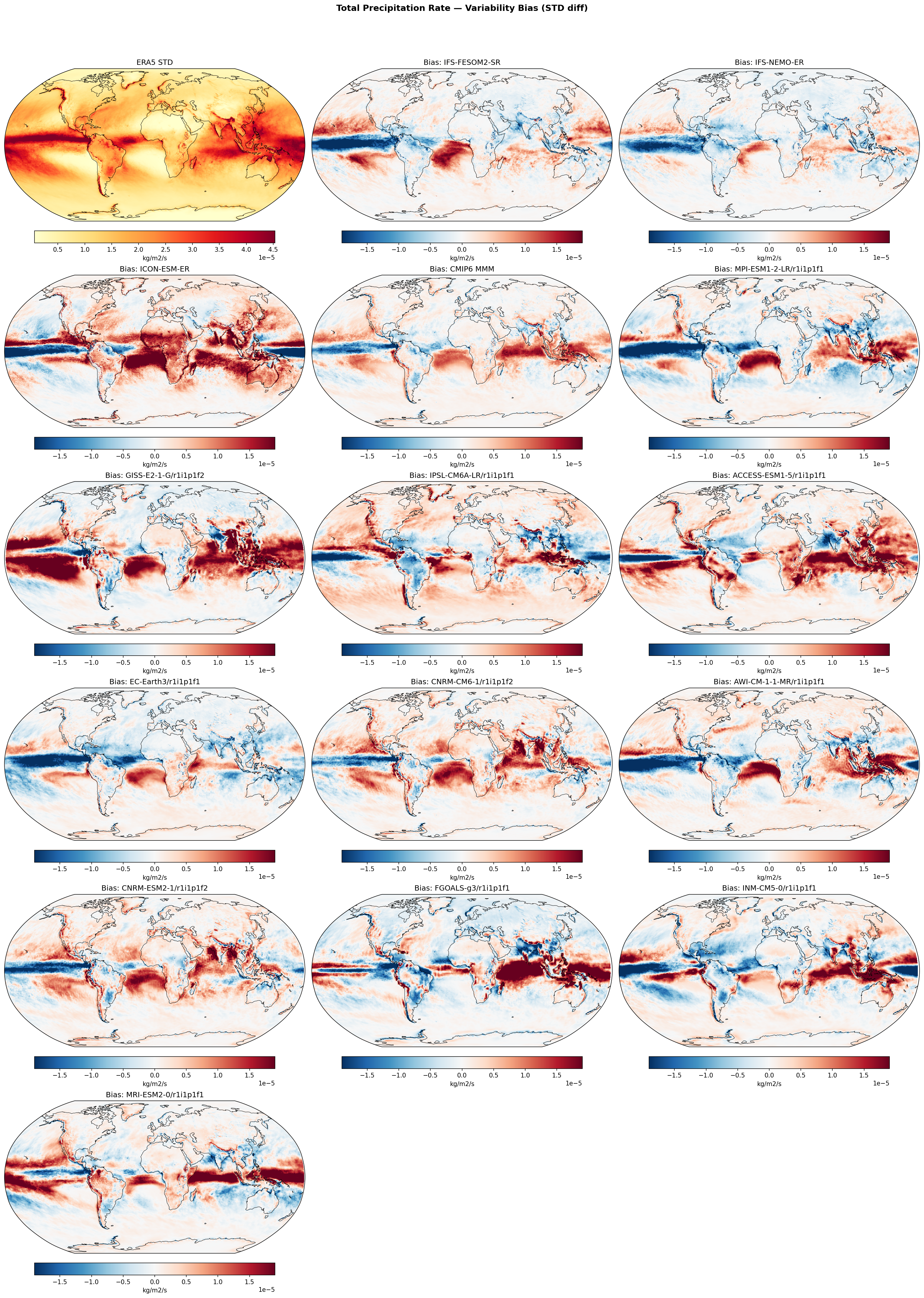
| Variables | pr |
|---|---|
| Models | IFS-FESOM2-SR, IFS-NEMO-ER, ICON-ESM-ER, HadGEM3-GC5, CMIP6 MMM, MPI-ESM1-2-LR/r1i1p1f1, GISS-E2-1-G/r1i1p1f2, IPSL-CM6A-LR/r1i1p1f1, ACCESS-ESM1-5/r1i1p1f1, EC-Earth3/r1i1p1f1, CNRM-CM6-1/r1i1p1f2, AWI-CM-1-1-MR/r1i1p1f1, CNRM-ESM2-1/r1i1p1f2, FGOALS-g3/r1i1p1f1, INM-CM5-0/r1i1p1f1, MRI-ESM2-0/r1i1p1f1 |
| Reference Dataset | ERA5 |
| Units | kg/m2/s |
| Period | 1980–2014 |
| IFS-FESOM2-SR | Std Gmean: 0.00 · Diff Gmean: 0.00 · Rmse: 0.00 |
| IFS-NEMO-ER | Std Gmean: 0.00 · Diff Gmean: -0.00 · Rmse: 0.00 |
| ICON-ESM-ER | Std Gmean: 0.00 · Diff Gmean: 0.00 · Rmse: 0.00 |
| HadGEM3-GC5 | Std Gmean: 0.00 · Diff Gmean: 0.00 · Rmse: 0.00 |
| CMIP6 MMM | Std Gmean: 0.00 · Diff Gmean: 0.00 · Rmse: 0.00 |
Summary high
This figure evaluates the variability of precipitation (standard deviation of monthly anomalies) in high-resolution EERIE models and CMIP6 against ERA5 reanalysis. It highlights systematic biases in the amplitude of tropical rainfall variability, particularly related to the placement and intensity of the Intertropical Convergence Zone (ITCZ).
Key Findings
- ICON-ESM-ER is a significant outlier, exhibiting widespread and strong overestimation of precipitation variability (red bias) across the global tropics, resulting in the highest RMSE (9.10e-6 kg/m²/s).
- A systematic 'Pacific Equatorial Dipole' bias is evident in most models (IFS, HadGEM3, and CMIP6 MMM): variability is underestimated along the equator (blue) but overestimated in flanking bands (red), a signature of the double-ITCZ bias.
- IFS-NEMO-ER demonstrates the lowest spatial RMSE (4.41e-6 kg/m²/s) among the EERIE models, showing a slight tendency to underestimate variability globally, whereas IFS-FESOM2-SR and HadGEM3-GC5 tend to overestimate it in off-equatorial regions.
Spatial Patterns
The dominant error structure is meridional in the Pacific: a band of suppressed variability along the equator (0°N) flanked by bands of excess variability at ~5-10°N and ~5-10°S. This corresponds to models anchoring convection off the equator. The Indian Ocean and SPCZ regions generally show excess variability (red) in most models, particularly in ICON-ESM-ER and GISS-E2-1-G. The Atlantic ITCZ also tends to show excess variability in the models.
Model Agreement
While magnitudes differ, there is strong structural agreement on the location of biases between the high-resolution EERIE models (excluding ICON) and the CMIP6 Multi-Model Mean. Both groups struggle with the equatorial Pacific. ICON-ESM-ER diverges by predicting much higher variability globally. IFS-NEMO-ER agrees best with ERA5 in terms of magnitude, though it shares the common spatial bias patterns.
Physical Interpretation
The underestimated variability along the Pacific equator likely stems from the 'cold tongue bias' common in coupled models; if the mean SST is too cold, the threshold for deep convection is rarely crossed, suppressing the intermittency and variance of rainfall (and potentially dampening ENSO-driven precipitation response). The excess variability in the off-equatorial bands (double ITCZ) suggests that models simulate a precipitation zone that is either too intense or shifts meridionally more than observed. ICON's widespread red bias suggests an overly sensitive convection scheme that triggers deep convection too frequently or with excessive intensity.
Caveats
- ERA5 precipitation is a model-derived product (reanalysis) and may contain its own biases, particularly in the tropical oceans.
- The analysis refers to monthly variability; sub-monthly or daily rainfall characteristics may differ.
Mean Sea Level Pressure — Variability (STD)
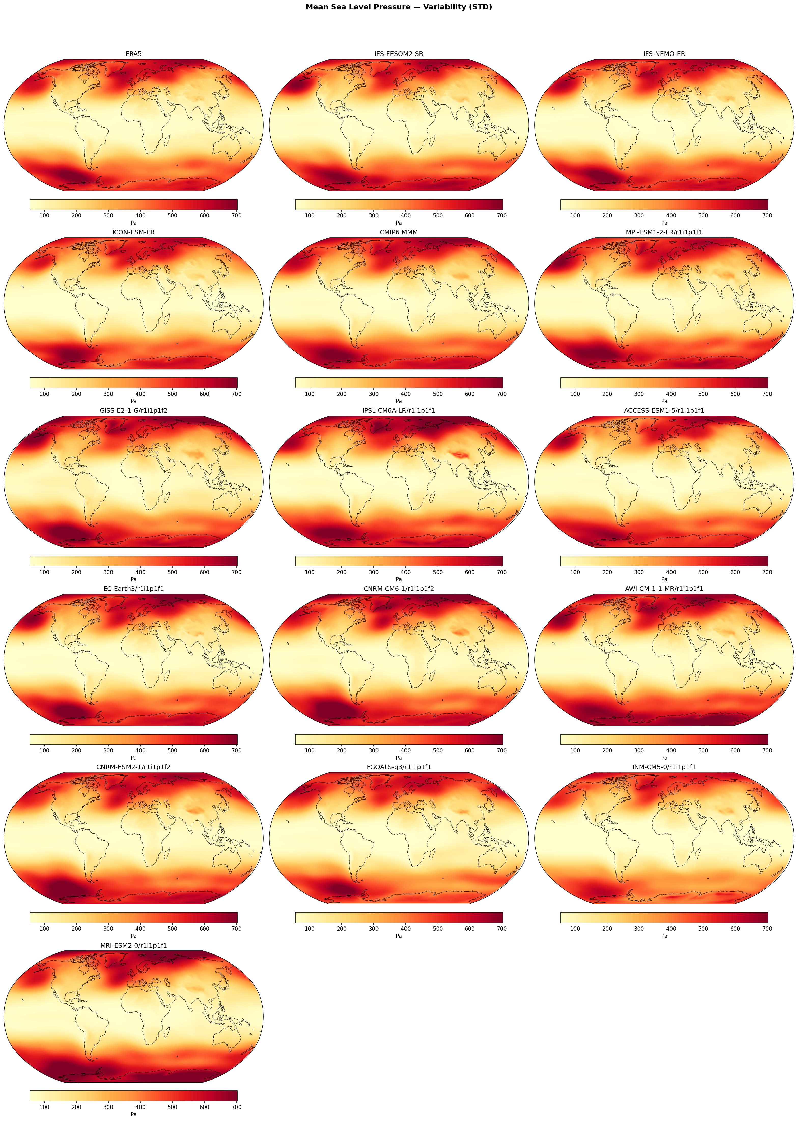
| Variables | psl |
|---|---|
| Models | IFS-FESOM2-SR, IFS-NEMO-ER, ICON-ESM-ER, CMIP6 MMM, MPI-ESM1-2-LR/r1i1p1f1, GISS-E2-1-G/r1i1p1f2, IPSL-CM6A-LR/r1i1p1f1, ACCESS-ESM1-5/r1i1p1f1, EC-Earth3/r1i1p1f1, CNRM-CM6-1/r1i1p1f2, AWI-CM-1-1-MR/r1i1p1f1, CNRM-ESM2-1/r1i1p1f2, FGOALS-g3/r1i1p1f1, INM-CM5-0/r1i1p1f1, MRI-ESM2-0/r1i1p1f1 |
| Reference Dataset | ERA5 |
| Units | Pa |
| Period | 1980–2014 |
| IFS-FESOM2-SR | Std Gmean: 239.35 · Diff Gmean: 3.56 · Rmse: 24.18 |
| IFS-NEMO-ER | Std Gmean: 239.05 · Diff Gmean: 3.26 · Rmse: 19.96 |
| ICON-ESM-ER | Std Gmean: 228.37 · Diff Gmean: -7.41 · Rmse: 32.64 |
| CMIP6 MMM | Std Gmean: 249.90 · Diff Gmean: 14.19 · Rmse: 26.38 |
Summary high
This figure compares the interannual variability of Mean Sea Level Pressure (PSL), quantified as the standard deviation of deseasonalised monthly anomalies, across high-resolution EERIE models, CMIP6 models, and ERA5 reanalysis. The high-resolution IFS simulations exhibit excellent agreement with observations, while ICON-ESM-ER underestimates variability and the CMIP6 ensemble mean slightly overestimates it.
Key Findings
- IFS-NEMO-ER and IFS-FESOM2-SR show high skill in reproducing observed variability patterns, with low global RMSEs (20.0 Pa and 24.2 Pa, respectively) and spatial structures nearly indistinguishable from ERA5.
- ICON-ESM-ER systematically underestimates PSL variability (global mean bias -7.4 Pa), particularly visible as reduced intensity in the Southern Ocean and North Atlantic storm tracks compared to ERA5.
- The CMIP6 Multi-Model Mean (MMM) generally overestimates variability (global bias +14.2 Pa), with significant spread among individual CMIP6 members (e.g., INM-CM5-0 is notably weak, while ACCESS-ESM1-5 is strong).
- Variability hotspots are correctly located in the mid-to-high latitude storm tracks, while tropical variability remains realistically low across most models.
Spatial Patterns
Dominant features are the zonal bands of high variability (>600 Pa) in the Southern Ocean and the localized maxima in the Northern Hemisphere storm tracks (Aleutian Low in N. Pacific, Icelandic Low in N. Atlantic). The tropics consistently show low variability (<200 Pa).
Model Agreement
The two IFS-based EERIE models (NEMO and FESOM2 backends) agree very closely with each other and ERA5. ICON-ESM-ER is an outlier among the EERIE set, showing weaker variance. The CMIP6 ensemble captures the main features but individual members show large divergence in amplitude.
Physical Interpretation
The patterns reflect the month-to-month variability associated with the major storm tracks and large-scale atmospheric modes (e.g., NAO, SAM, PNA). High variability in the extratropics arises from baroclinic instability and the resulting cyclone activity, which shifts substantially on monthly timescales. The high resolution of the EERIE models likely contributes to better resolving the intensity of these dynamical features compared to the lower-resolution outliers in CMIP6, although the underestimation in ICON suggests tuning or dynamical core differences also play a role.
Caveats
- The metric uses monthly means, so it conflates interannual variability of the mean flow with the integrated effect of synoptic storminess; it does not directly measure high-frequency storm intensity.
- CMIP6 MMM smoothness masks the extreme biases of individual members visible in the lower panels.
Mean Sea Level Pressure — Variability Bias (STD diff)
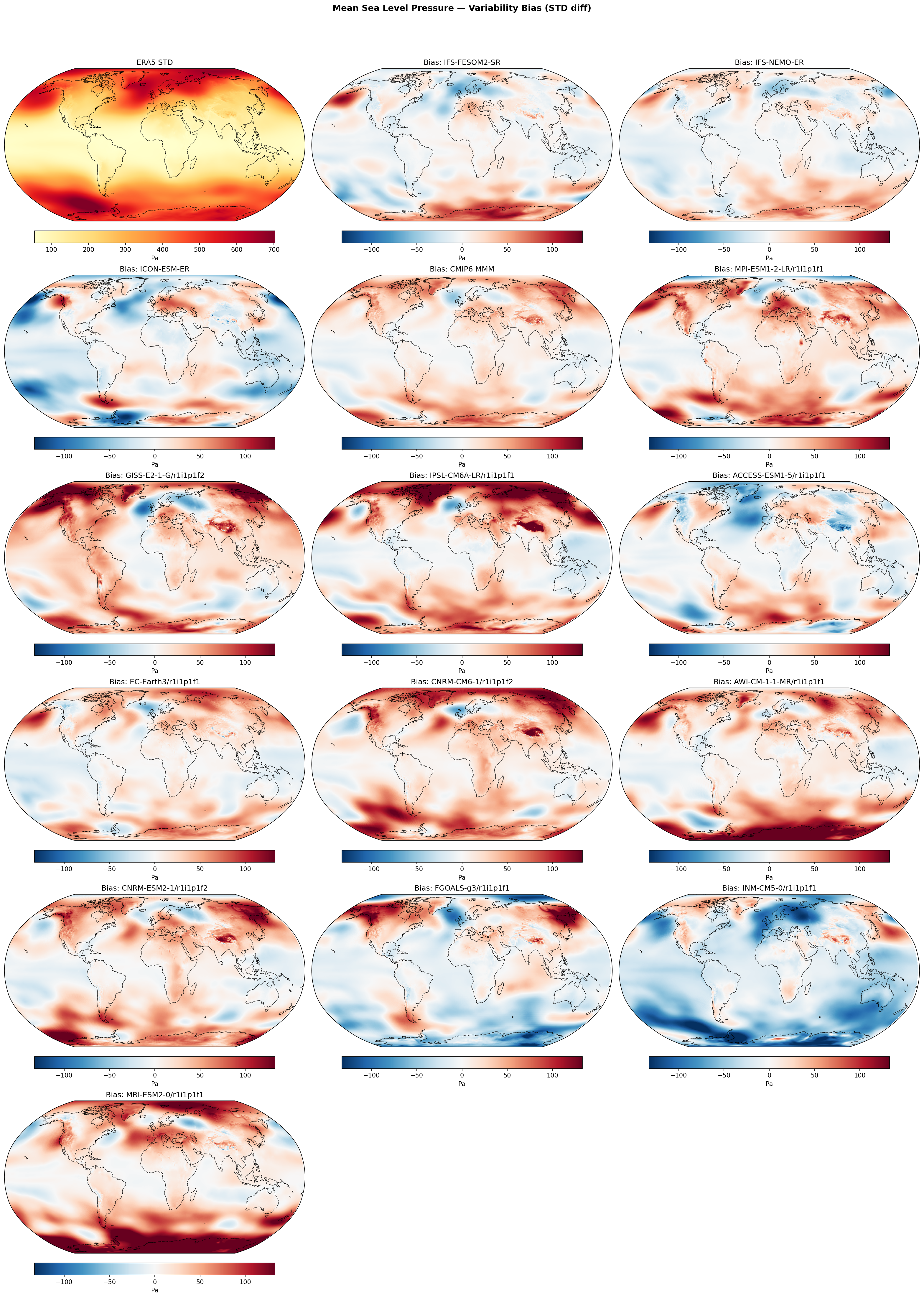
| Variables | psl |
|---|---|
| Models | IFS-FESOM2-SR, IFS-NEMO-ER, ICON-ESM-ER, CMIP6 MMM, MPI-ESM1-2-LR/r1i1p1f1, GISS-E2-1-G/r1i1p1f2, IPSL-CM6A-LR/r1i1p1f1, ACCESS-ESM1-5/r1i1p1f1, EC-Earth3/r1i1p1f1, CNRM-CM6-1/r1i1p1f2, AWI-CM-1-1-MR/r1i1p1f1, CNRM-ESM2-1/r1i1p1f2, FGOALS-g3/r1i1p1f1, INM-CM5-0/r1i1p1f1, MRI-ESM2-0/r1i1p1f1 |
| Reference Dataset | ERA5 |
| Units | Pa |
| Period | 1980–2014 |
| IFS-FESOM2-SR | Std Gmean: 239.35 · Diff Gmean: 3.56 · Rmse: 24.18 |
| IFS-NEMO-ER | Std Gmean: 239.05 · Diff Gmean: 3.26 · Rmse: 19.96 |
| ICON-ESM-ER | Std Gmean: 228.37 · Diff Gmean: -7.41 · Rmse: 32.64 |
| CMIP6 MMM | Std Gmean: 249.90 · Diff Gmean: 14.19 · Rmse: 26.38 |
Summary high
This figure evaluates the variability of Mean Sea Level Pressure (PSL) by comparing the standard deviation (STD) of monthly anomalies in models against ERA5 reanalysis. It highlights a distinct performance gap: IFS-based high-resolution models closely match observed variability, ICON-ESM-ER underestimates it, and the CMIP6 ensemble generally overestimates it.
Key Findings
- IFS-NEMO-ER and IFS-FESOM2-SR exhibit excellent skill, showing the lowest RMSE (~20-24 Pa) and very weak spatial bias patterns, indicating they correctly capture the intensity of synoptic-scale variability.
- ICON-ESM-ER displays a systematic negative bias (blue) globally, significantly underestimating variability in the major storm tracks (North Pacific, Southern Ocean) with a global mean deficit of -7.4 Pa.
- The CMIP6 Multi-Model Mean (MMM) and many individual CMIP6 models (e.g., GISS-E2-1-G, CNRM-CM6-1) tend to overestimate PSL variability (red), particularly over Northern Hemisphere continents and the Arctic.
- Southern Ocean storm track variability is robustly captured by ERA5 and IFS models, but severely damped in ICON-ESM-ER and spatially displaced or exaggerated in several CMIP6 models.
Spatial Patterns
ERA5 shows characteristic bands of high variability (>500 Pa) in the extratropical storm tracks (North Atlantic, North Pacific, Southern Ocean). Biases in the IFS models are patchy and low-magnitude (<50 Pa). ICON shows widespread negative biases (underestimation) exceeding -100 Pa in storm track regions. CMIP6 models show large positive biases (>100 Pa) over NH landmasses and the Arctic, with complex dipole biases in the Southern Ocean suggesting latitudinal shifts in the storm track.
Model Agreement
There is strong agreement between the two IFS variants (NEMO vs FESOM2), which both align well with ERA5. There is significant divergence between the high-resolution groups (IFS vs ICON) and widespread disagreement within the CMIP6 ensemble, ranging from severe underestimation (INM-CM5-0) to severe overestimation (GISS-E2-1-G).
Physical Interpretation
PSL variability is a proxy for synoptic-scale cyclone and anticyclone activity (storm tracks). The high-resolution IFS dynamics appear effective at generating realistic storm intensity without excessive damping. In contrast, ICON-ESM-ER appears overly diffusive or damped, suppressing storm track variance. The excess variability in coarser CMIP6 models may stem from circulation biases, such as overly persistent blocking events or deeper-than-observed low-pressure systems, rather than resolution alone.
Caveats
- Biases over high topography (Antarctica, Himalayas, Greenland) should be interpreted with caution due to errors inherent in reducing surface pressure to sea level.
- The figure uses monthly data standard deviations, which aggregates synoptic (weather) and lower-frequency variability; it does not distinguish between storm frequency and storm intensity.
Surface Downwelling Longwave — Variability (STD)
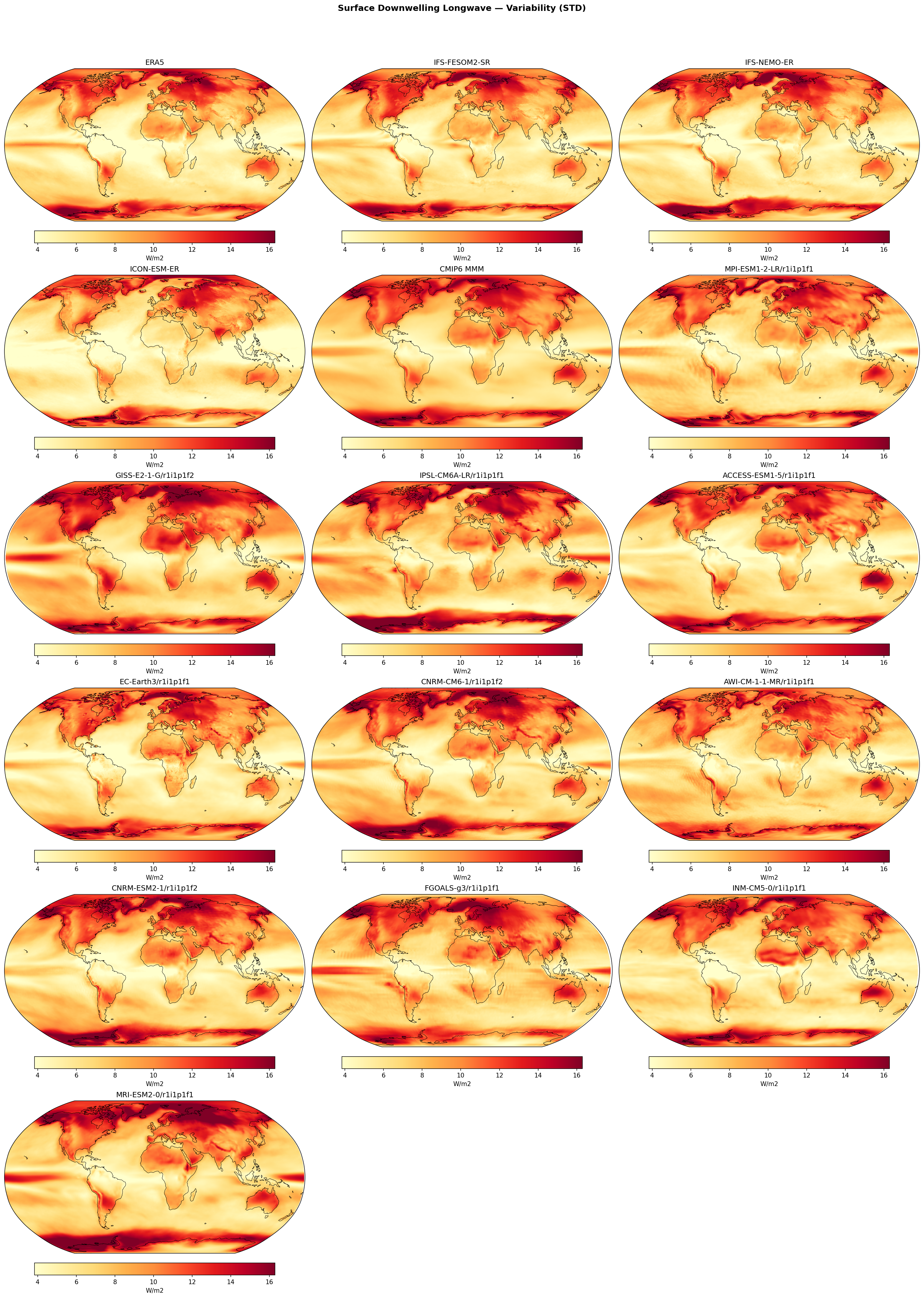
| Variables | rlds |
|---|---|
| Models | IFS-FESOM2-SR, IFS-NEMO-ER, ICON-ESM-ER, CMIP6 MMM, MPI-ESM1-2-LR/r1i1p1f1, GISS-E2-1-G/r1i1p1f2, IPSL-CM6A-LR/r1i1p1f1, ACCESS-ESM1-5/r1i1p1f1, EC-Earth3/r1i1p1f1, CNRM-CM6-1/r1i1p1f2, AWI-CM-1-1-MR/r1i1p1f1, CNRM-ESM2-1/r1i1p1f2, FGOALS-g3/r1i1p1f1, INM-CM5-0/r1i1p1f1, MRI-ESM2-0/r1i1p1f1 |
| Reference Dataset | ERA5 |
| Units | W/m2 |
| Period | 1980–2014 |
| IFS-FESOM2-SR | Std Gmean: 7.48 · Diff Gmean: 0.31 · Rmse: 1.11 |
| IFS-NEMO-ER | Std Gmean: 7.31 · Diff Gmean: 0.14 · Rmse: 0.99 |
| ICON-ESM-ER | Std Gmean: 6.72 · Diff Gmean: -0.45 · Rmse: 1.74 |
| CMIP6 MMM | Std Gmean: 8.11 · Diff Gmean: 0.94 · Rmse: 1.34 |
Summary high
This diagnostic shows the standard deviation of deseasonalised, detrended surface downwelling longwave radiation, serving as a metric for internal climate variability. The high-resolution IFS models closely reproduce the variability patterns seen in ERA5, whereas ICON-ESM-ER underestimates variability and CMIP6 models generally overestimate it.
Key Findings
- IFS-NEMO-ER shows the highest skill in reproducing ERA5 variability (RMSE 0.99 W/m²), closely followed by IFS-FESOM2-SR (RMSE 1.11 W/m²), capturing both the spatial structure and magnitude.
- ICON-ESM-ER systematically underestimates variability (global mean difference -0.45 W/m²), with noticeably paler patterns over the tropical oceans and weaker ENSO-related variance.
- CMIP6 models exhibit a wide spread in variability amplitude, with the Multi-Model Mean (MMM) overestimating variability by ~0.94 W/m² globally; individual models like GISS-E2-1-G show excessive variability in polar regions.
Spatial Patterns
The strongest variability (>14 W/m²) occurs over Northern Hemisphere land masses (North America, Eurasia) and the Southern Ocean margins, reflecting large synoptic temperature and cloud variations. In the tropics, a distinct band of high variability spans the equatorial Pacific, associated with ENSO-driven fluctuations in atmospheric moisture and convection. Subtropical gyres show the lowest variability.
Model Agreement
The two IFS variants agree strongly with each other and ERA5. ICON-ESM-ER is an outlier among the EERIE models with dampened variability. The CMIP6 ensemble shows substantial inter-model divergence, particularly in the magnitude of variability over high-latitude land and oceans.
Physical Interpretation
Downwelling longwave variability is driven by variations in near-surface air temperature and effective atmospheric emissivity (cloud cover and water vapor). High variability over land results from the low heat capacity of the surface allowing large temperature swings. Tropical patterns are driven by the displacement of deep convection and moisture anomalies (e.g., during El Niño/La Niña events).
Caveats
- The reference dataset, ERA5, is a reanalysis product and its radiative fluxes are model-derived.
- The analysis depends on the effectiveness of the detrending and deseasonalising process to isolate internal variability.
Surface Downwelling Longwave — Variability Bias (STD diff)
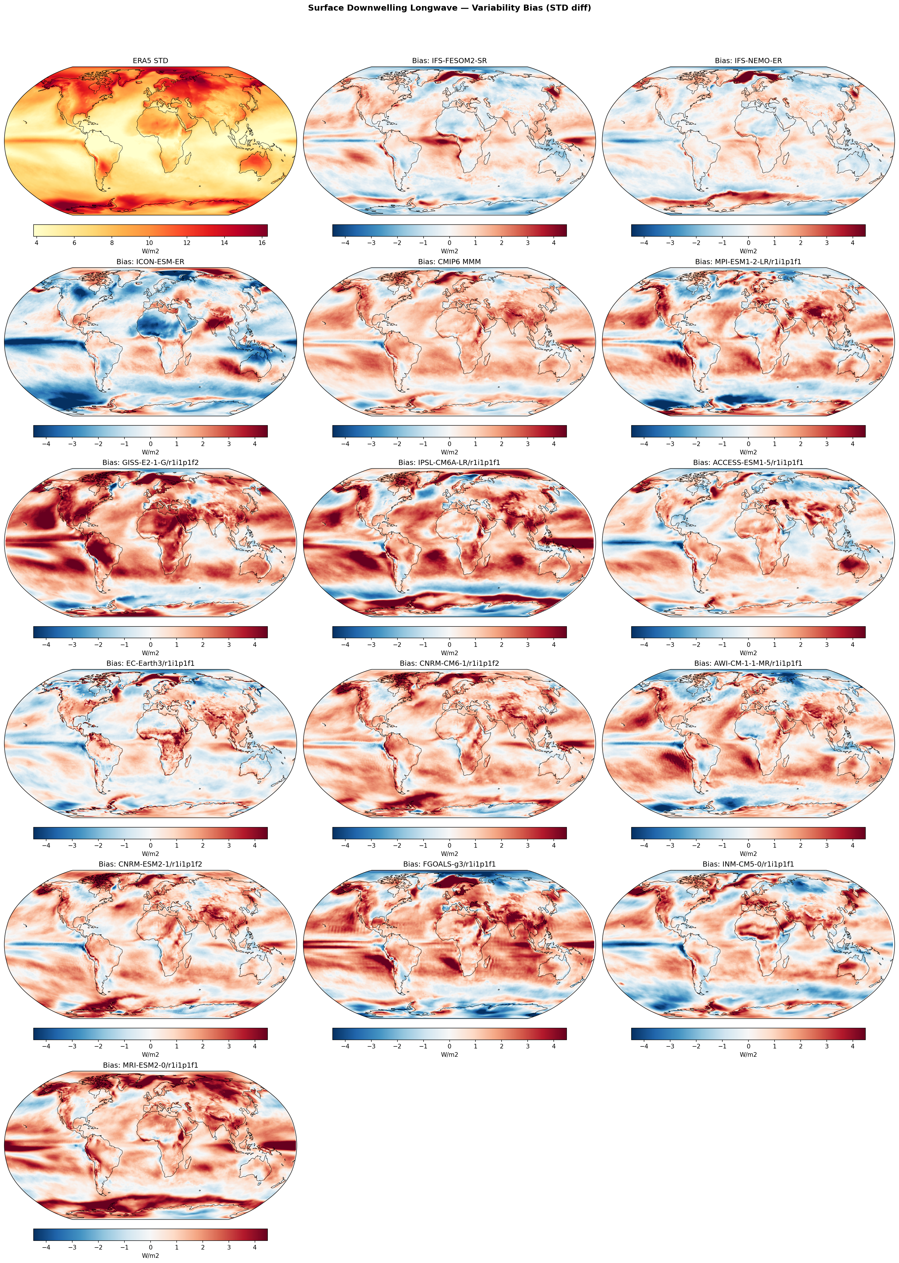
| Variables | rlds |
|---|---|
| Models | IFS-FESOM2-SR, IFS-NEMO-ER, ICON-ESM-ER, CMIP6 MMM, MPI-ESM1-2-LR/r1i1p1f1, GISS-E2-1-G/r1i1p1f2, IPSL-CM6A-LR/r1i1p1f1, ACCESS-ESM1-5/r1i1p1f1, EC-Earth3/r1i1p1f1, CNRM-CM6-1/r1i1p1f2, AWI-CM-1-1-MR/r1i1p1f1, CNRM-ESM2-1/r1i1p1f2, FGOALS-g3/r1i1p1f1, INM-CM5-0/r1i1p1f1, MRI-ESM2-0/r1i1p1f1 |
| Reference Dataset | ERA5 |
| Units | W/m2 |
| Period | 1980–2014 |
| IFS-FESOM2-SR | Std Gmean: 7.48 · Diff Gmean: 0.31 · Rmse: 1.11 |
| IFS-NEMO-ER | Std Gmean: 7.31 · Diff Gmean: 0.14 · Rmse: 0.99 |
| ICON-ESM-ER | Std Gmean: 6.72 · Diff Gmean: -0.45 · Rmse: 1.74 |
| CMIP6 MMM | Std Gmean: 8.11 · Diff Gmean: 0.94 · Rmse: 1.34 |
Summary high
This diagnostic evaluates the variability of surface downwelling longwave radiation (rlds) by comparing the standard deviation of monthly anomalies in models versus ERA5. The high-resolution IFS-based models demonstrate superior skill with low biases, whereas the CMIP6 ensemble generally overestimates variability and ICON-ESM-ER tends to underestimate it in the extratropics.
Key Findings
- IFS-NEMO-ER and IFS-FESOM2-SR show the best agreement with observations (RMSE ~1.0-1.1 W/m²), exhibiting significantly lower biases than the CMIP6 Multi-Model Mean.
- The CMIP6 MMM and most individual CMIP6 models display a widespread positive bias (red), indicating excessive variability in downwelling longwave radiation, particularly over the Tropical Pacific and Southern Ocean.
- ICON-ESM-ER shows a distinct negative bias (blue) over the North Atlantic, North Pacific, and Eurasia, indicating it underestimates the natural variability of longwave radiation in these regions.
Spatial Patterns
ERA5 shows peak variability over high-latitude land masses and the Southern Ocean. The IFS models capture this well but show slight underestimation in eastern boundary upwelling regions (stratocumulus decks) and slight overestimation in the ENSO region. ICON-ESM-ER diverges with strong negative biases in the storm tracks. FGOALS-g3 exhibits visible horizontal striping artifacts.
Model Agreement
The two IFS variants (FESOM and NEMO) agree closely with each other and observations. There is a strong divergence between the CMIP6 ensemble (systematic overestimation) and ICON-ESM-ER (systematic underestimation in extratropics).
Physical Interpretation
Variability in surface downwelling longwave is primarily driven by fluctuations in cloud cover (cloud radiative effects) and lower tropospheric water vapor/temperature. The excessive variability in CMIP6 suggests overly volatile cloud regimes or exaggerated internal climate modes (e.g., ENSO). Conversely, ICON's underestimation in the storm tracks implies overly persistent cloud cover or dampened synoptic-scale variability.
Caveats
- ERA5 reanalysis relies on its own radiative transfer scheme, serving as a model-based reference.
- FGOALS-g3 displays numerical or regridding artifacts (horizontal striations) that compromise its physical representation.
Surface Downwelling Shortwave — Variability (STD)
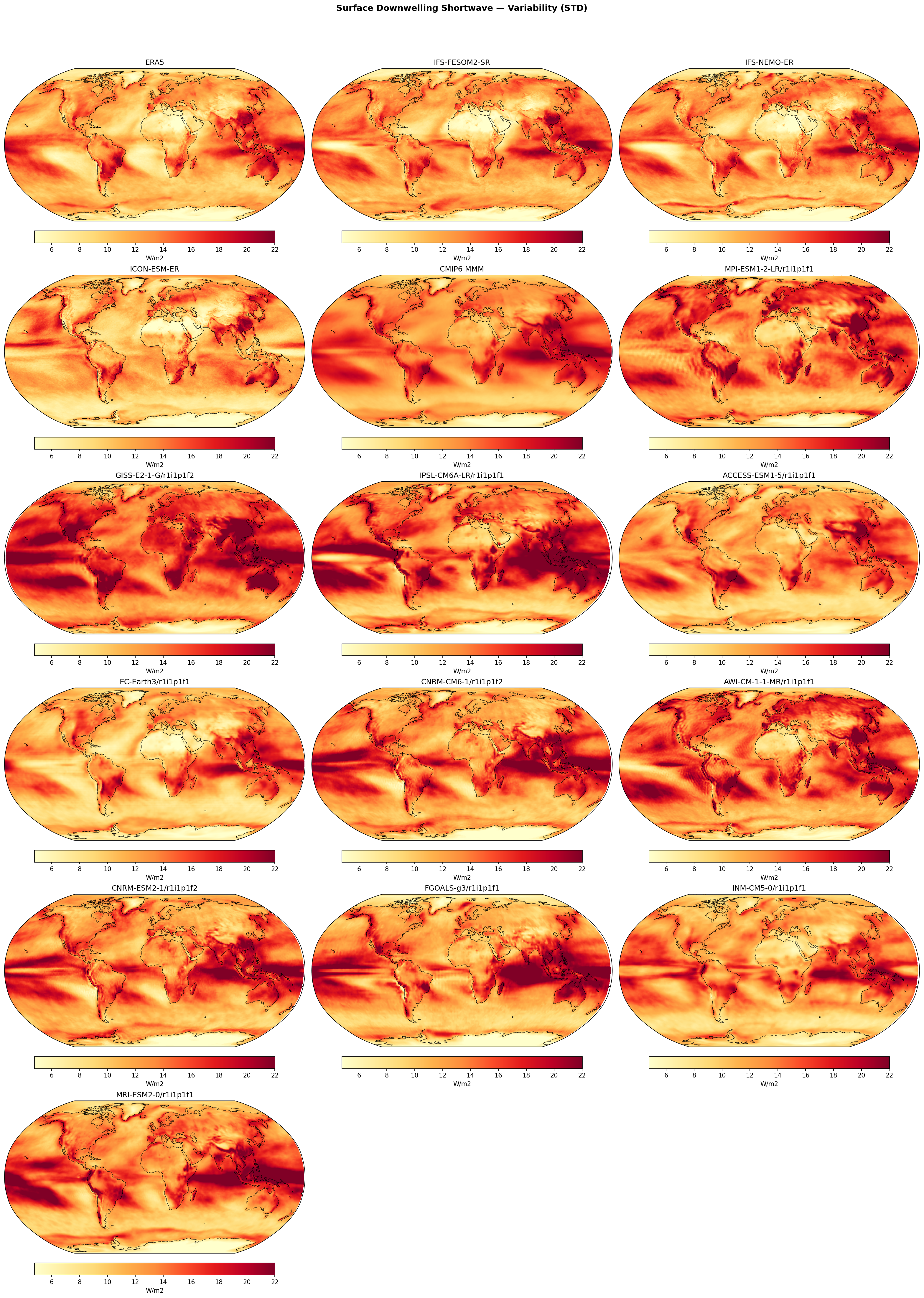
| Variables | rsds |
|---|---|
| Models | IFS-FESOM2-SR, IFS-NEMO-ER, ICON-ESM-ER, CMIP6 MMM, MPI-ESM1-2-LR/r1i1p1f1, GISS-E2-1-G/r1i1p1f2, IPSL-CM6A-LR/r1i1p1f1, ACCESS-ESM1-5/r1i1p1f1, EC-Earth3/r1i1p1f1, CNRM-CM6-1/r1i1p1f2, AWI-CM-1-1-MR/r1i1p1f1, CNRM-ESM2-1/r1i1p1f2, FGOALS-g3/r1i1p1f1, INM-CM5-0/r1i1p1f1, MRI-ESM2-0/r1i1p1f1 |
| Reference Dataset | ERA5 |
| Units | W/m2 |
| Period | 1980–2014 |
| IFS-FESOM2-SR | Std Gmean: 12.40 · Diff Gmean: 0.49 · Rmse: 2.25 |
| IFS-NEMO-ER | Std Gmean: 12.30 · Diff Gmean: 0.40 · Rmse: 1.94 |
| ICON-ESM-ER | Std Gmean: 11.38 · Diff Gmean: -0.53 · Rmse: 3.33 |
| CMIP6 MMM | Std Gmean: 13.97 · Diff Gmean: 2.07 · Rmse: 2.88 |
Summary high
This diagnostic compares the standard deviation of deseasonalised, detrended surface downwelling shortwave radiation (rsds) across high-resolution EERIE simulations (IFS, ICON) and CMIP6 models against ERA5 reanalysis. The analysis reveals that the IFS-based high-resolution models capture observed variability patterns with high fidelity, whereas CMIP6 models exhibit large biases and inter-model spread.
Key Findings
- IFS-NEMO-ER and IFS-FESOM2-SR show excellent agreement with ERA5, with IFS-NEMO-ER achieving the lowest RMSE (1.94 W/m²) and accurately reproducing variability in the ENSO region and storm tracks.
- The CMIP6 Multi-Model Mean (MMM) and several individual CMIP6 models (e.g., GISS-E2-1-G, IPSL-CM6A-LR) significantly overestimate surface SW variability (MMM global mean ~14.0 W/m² vs. IFS/ERA5 ~12.3 W/m²).
- ICON-ESM-ER systematically underestimates variability (global mean ~11.4 W/m², negative bias), particularly damping the signal in the tropical Pacific and storm tracks compared to ERA5.
Spatial Patterns
Dominant features include high variability in the central/eastern Tropical Pacific (associated with ENSO-driven cloud shifts), the Indo-Pacific Warm Pool, and mid-latitude storm tracks (North Atlantic, North Pacific, Southern Ocean). Land regions with strong convective activity (Amazon, Congo) also show local maxima. The CMIP6 MMM tends to smear the tropical Pacific signal zonally compared to the more confined 'tongue' structure in ERA5 and IFS models.
Model Agreement
There is strong agreement between ERA5 and the two IFS models (FESOM and NEMO), which effectively capture the magnitude and location of cloud-induced variability. In contrast, CMIP6 models diverge widely: GISS and IPSL show excessive 'flashiness' (global red bias), while INM-CM5-0 and FGOALS-g3 show muted variability. ICON-ESM-ER is an outlier among the high-resolution group, showing weaker variability than observed.
Physical Interpretation
Surface SW variability is primarily a proxy for cloud cover variability (Cloud Radiative Effect). The high variability in the tropical Pacific reflects ENSO-related shifts in convection, while mid-latitude bands reflect synoptic storm passage. The superior performance of IFS models suggests that high spatial resolution improves the representation of synoptic cloud systems and their temporal evolution. Conversely, the excessive variability in some CMIP6 models likely stems from convective parameterisations that trigger precipitation/clouds too intermittently ('on/off' behaviour) or overestimate the radiative impact of cloud anomalies.
Caveats
- ERA5 surface radiation is model-derived (though constrained by data assimilation) and not a direct observation like CERES, though spatial patterns are generally robust.
- The metric combines variability from multiple timescales (monthly to multi-decadal); ENSO dominates the tropical Pacific signal, so biases there may reflect ENSO amplitude biases rather than just cloud physics.
Surface Downwelling Shortwave — Variability Bias (STD diff)
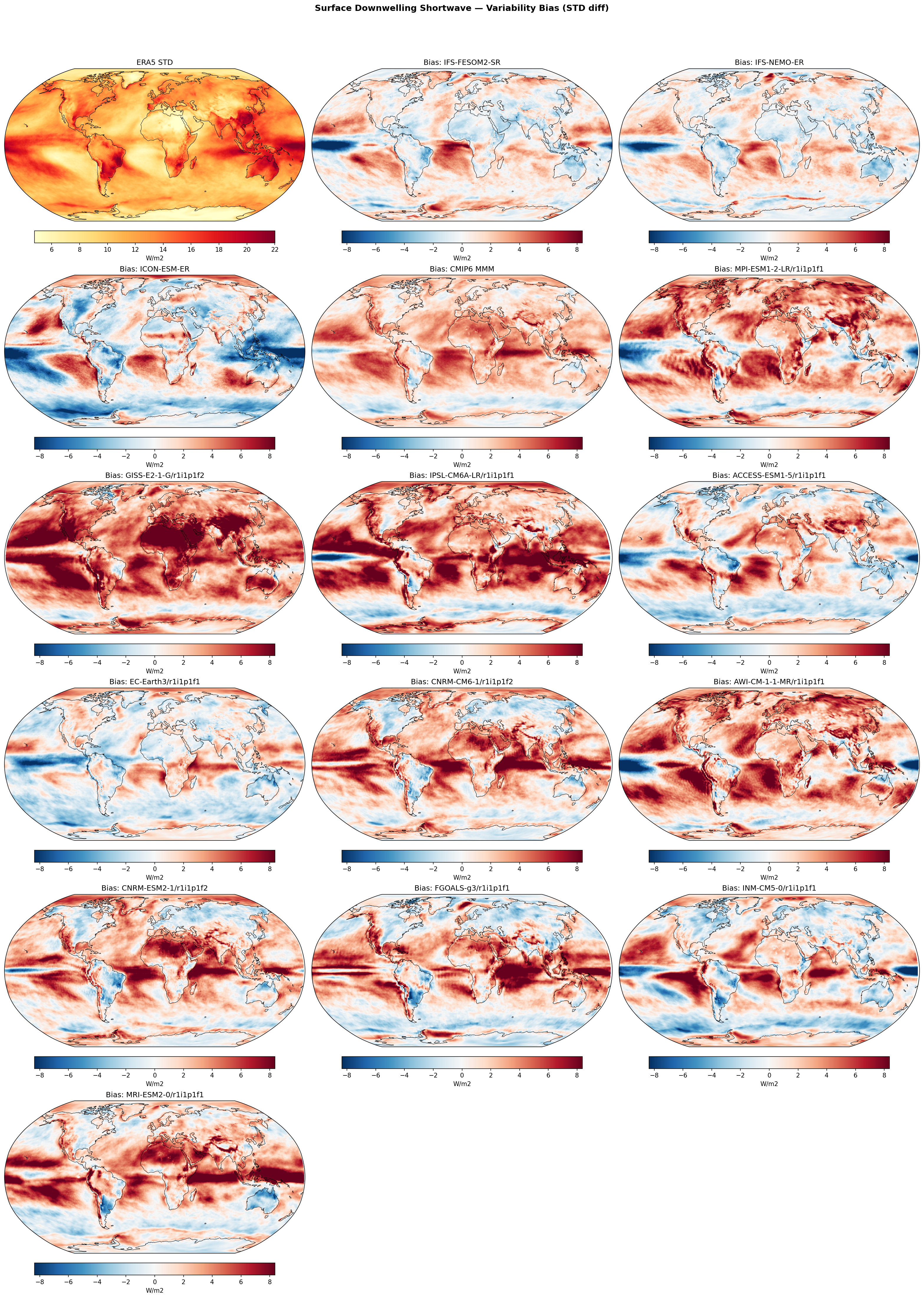
| Variables | rsds |
|---|---|
| Models | IFS-FESOM2-SR, IFS-NEMO-ER, ICON-ESM-ER, CMIP6 MMM, MPI-ESM1-2-LR/r1i1p1f1, GISS-E2-1-G/r1i1p1f2, IPSL-CM6A-LR/r1i1p1f1, ACCESS-ESM1-5/r1i1p1f1, EC-Earth3/r1i1p1f1, CNRM-CM6-1/r1i1p1f2, AWI-CM-1-1-MR/r1i1p1f1, CNRM-ESM2-1/r1i1p1f2, FGOALS-g3/r1i1p1f1, INM-CM5-0/r1i1p1f1, MRI-ESM2-0/r1i1p1f1 |
| Reference Dataset | ERA5 |
| Units | W/m2 |
| Period | 1980–2014 |
| IFS-FESOM2-SR | Std Gmean: 12.40 · Diff Gmean: 0.49 · Rmse: 2.25 |
| IFS-NEMO-ER | Std Gmean: 12.30 · Diff Gmean: 0.40 · Rmse: 1.94 |
| ICON-ESM-ER | Std Gmean: 11.38 · Diff Gmean: -0.53 · Rmse: 3.33 |
| CMIP6 MMM | Std Gmean: 13.97 · Diff Gmean: 2.07 · Rmse: 2.88 |
Summary high
This diagnostic evaluates the variability (standard deviation of monthly anomalies) of surface downwelling shortwave radiation. The high-resolution IFS models (IFS-NEMO-ER and IFS-FESOM2-SR) show superior skill in reproducing observed variability patterns compared to ICON-ESM-ER and the CMIP6 ensemble, which exhibit widespread under- and over-estimation respectively.
Key Findings
- IFS-NEMO-ER and IFS-FESOM2-SR demonstrate the best agreement with ERA5, with low RMSEs (1.94 and 2.25 W/m²) and relatively neutral spatial bias patterns.
- ICON-ESM-ER significantly underestimates shortwave variability over most global oceans (blue bias), particularly in the tropical and subtropical bands.
- The CMIP6 Multi-Model Mean and most individual CMIP6 models (e.g., GISS-E2-1-G, AWI-CM-1-1-MR) consistently overestimate surface shortwave variability (red bias), with the MMM showing a global mean positive bias of ~2.07 W/m².
Spatial Patterns
In ERA5, peak variability occurs in the Tropical Pacific (ENSO region), ITCZ, and mid-latitude storm tracks. The IFS models capture these features well but slightly underestimate variability in the central Tropical Pacific. ICON shows a strong negative bias across the tropics and subtropics. CMIP6 models show excessive variability in the Tropical Pacific, Southern Ocean, and over many land masses (e.g., Amazon, Africa).
Model Agreement
There is a distinct divergence between model groups: IFS models agree well with ERA5; ICON acts as an outlier with suppressed variability; and the CMIP6 ensemble generally exhibits excessive variability. Individual CMIP6 models like GISS-E2-1-G show extreme widespread positive biases.
Physical Interpretation
Surface shortwave variability is primarily driven by fluctuations in cloud cover. The underestimation in the central Pacific by IFS and ICON suggests either dampened ENSO amplitude or a weak cloud radiative response to SST anomalies in these runs. The widespread positive bias in CMIP6 models suggests 'flickering' convection or overly sensitive cloud radiative effects, where cloud fraction or optical depth varies too dramatically compared to the reanalysis baseline.
Caveats
- ERA5 surface radiation is a model-derived product (reanalysis) rather than direct satellite observation, though it generally assimilates relevant atmospheric data.
- Standard deviation biases reflect errors in the amplitude of climate variations (weather, ENSO, seasonal shifts) rather than mean state errors.
2m Temperature — Variability (STD)
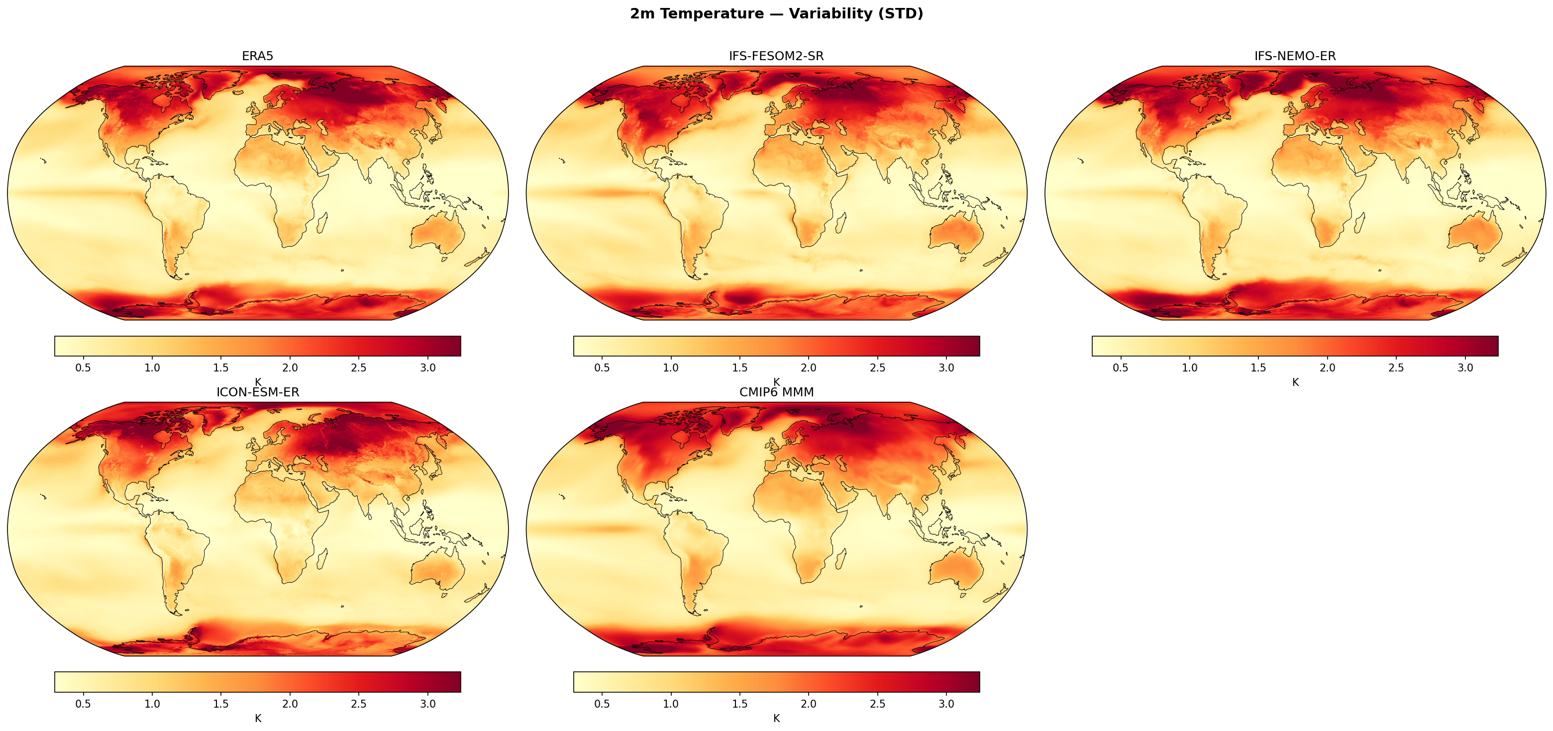
| Variables | tas |
|---|---|
| Models | IFS-FESOM2-SR, IFS-NEMO-ER, ICON-ESM-ER, HadGEM3-GC5, CMIP6 MMM, MPI-ESM1-2-LR/r1i1p1f1, GISS-E2-1-G/r1i1p1f2, IPSL-CM6A-LR/r1i1p1f1, ACCESS-ESM1-5/r1i1p1f1, EC-Earth3/r1i1p1f1, CNRM-CM6-1/r1i1p1f2, AWI-CM-1-1-MR/r1i1p1f1, CNRM-ESM2-1/r1i1p1f2, FGOALS-g3/r1i1p1f1, INM-CM5-0/r1i1p1f1, MRI-ESM2-0/r1i1p1f1 |
| Reference Dataset | ERA5 |
| Units | K |
| Period | 1980–2014 |
| IFS-FESOM2-SR | Std Gmean: 1.04 · Diff Gmean: 0.06 · Rmse: 0.21 |
| IFS-NEMO-ER | Std Gmean: 1.02 · Diff Gmean: 0.05 · Rmse: 0.22 |
| ICON-ESM-ER | Std Gmean: 0.95 · Diff Gmean: -0.02 · Rmse: 0.28 |
| HadGEM3-GC5 | Std Gmean: 0.98 · Diff Gmean: 0.00 · Rmse: 0.24 |
| CMIP6 MMM | Std Gmean: 1.05 · Diff Gmean: 0.08 · Rmse: 0.18 |
Summary high
The figure illustrates the standard deviation of deseasonalised, detrended monthly 2m temperature anomalies, highlighting global patterns of climate variability including the land-sea contrast, polar amplification, and the ENSO signature in the tropical Pacific. The high-resolution EERIE models generally reproduce the observed spatial structure of variability well, though with notable differences in the amplitude of tropical and polar features compared to ERA5 and the CMIP6 ensemble.
Key Findings
- **Land-Sea Contrast:** All models accurately capture the fundamental physical distinction where land surfaces (low heat capacity) exhibit much higher variability (2.0–3.0 K) than oceans (<1.0 K).
- **ENSO Representation:** The distinct 'tongue' of variability in the eastern tropical Pacific (characteristic of ENSO) is well-defined in IFS-FESOM2-SR, IFS-NEMO-ER, and HadGEM3-GC5, matching ERA5. In contrast, ICON-ESM-ER shows a noticeably weaker ENSO signature, suggesting suppressed tropical coupled variability.
- **High-Latitude Variance:** Variability is maximized in high-latitude continental regions (Siberia, North America) and sea-ice margins. While EERIE models generally align with ERA5, some individual CMIP6 models (e.g., IPSL-CM6A-LR, FGOALS-g3) exhibit excessive variability (>3 K) in the Arctic, likely indicative of sea-ice or boundary layer biases.
Spatial Patterns
The dominant spatial feature is the stark contrast between continental interiors (high variability) and open oceans (low variability). Superimposed on this are the enhanced variability at the sea-ice edges (both Arctic and Antarctic) and the ENSO wave train in the Pacific. ERA5 shows a specific pattern of variability over the Southern Ocean sea-ice zone which is generally well-reproduced by the EERIE models.
Model Agreement
HadGEM3-GC5 exhibits the best agreement with ERA5 in terms of global mean variability (diff_gmean: 0.003 K). The IFS models (FESOM2 and NEMO) slightly overestimate global variability (~+0.05 K) but capture spatial features robustly. ICON-ESM-ER is the outlier among EERIE simulations, underestimating global variability (-0.02 K) and showing the highest RMSE (0.27 K), largely due to the dampened tropical signal. The CMIP6 Multi-Model Mean (MMM) is smoother than individual realizations but has the lowest RMSE (0.17 K) due to error cancellation.
Physical Interpretation
The patterns are driven by surface heat capacity differences (land vs. ocean) and surface energy balance regimes. High variability over sea-ice margins results from the intermittency of insulating ice cover versus open ocean heat release. The tropical Pacific signal is driven by the Bjerknes feedback (ENSO). The excessive Arctic variability in some models points to issues with stable boundary layer parameterisations or excessive sensitivity of sea ice to forcing.
Caveats
- The use of monthly means filters out high-frequency synoptic variability, focusing the analysis on interannual and seasonal-scale variance.
- CMIP6 MMM smoothness is an artifact of averaging multiple realizations, artificially dampening internal variability compared to single-realization EERIE runs.
2m Temperature — Variability Bias (STD diff)
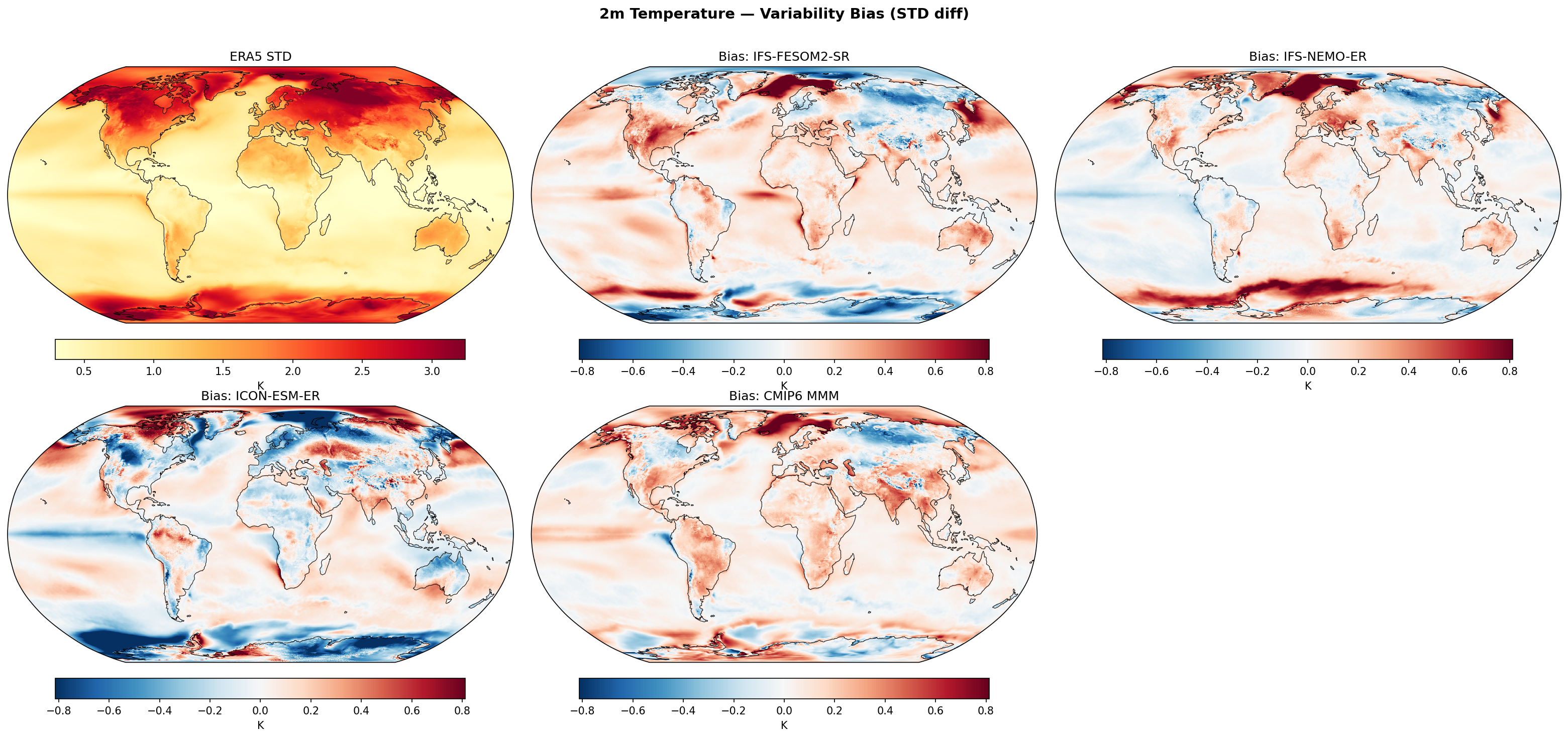
| Variables | tas |
|---|---|
| Models | IFS-FESOM2-SR, IFS-NEMO-ER, ICON-ESM-ER, HadGEM3-GC5, CMIP6 MMM, MPI-ESM1-2-LR/r1i1p1f1, GISS-E2-1-G/r1i1p1f2, IPSL-CM6A-LR/r1i1p1f1, ACCESS-ESM1-5/r1i1p1f1, EC-Earth3/r1i1p1f1, CNRM-CM6-1/r1i1p1f2, AWI-CM-1-1-MR/r1i1p1f1, CNRM-ESM2-1/r1i1p1f2, FGOALS-g3/r1i1p1f1, INM-CM5-0/r1i1p1f1, MRI-ESM2-0/r1i1p1f1 |
| Reference Dataset | ERA5 |
| Units | K |
| Period | 1980–2014 |
| IFS-FESOM2-SR | Std Gmean: 1.04 · Diff Gmean: 0.06 · Rmse: 0.21 |
| IFS-NEMO-ER | Std Gmean: 1.02 · Diff Gmean: 0.05 · Rmse: 0.22 |
| ICON-ESM-ER | Std Gmean: 0.95 · Diff Gmean: -0.02 · Rmse: 0.28 |
| HadGEM3-GC5 | Std Gmean: 0.98 · Diff Gmean: 0.00 · Rmse: 0.24 |
| CMIP6 MMM | Std Gmean: 1.05 · Diff Gmean: 0.08 · Rmse: 0.18 |
Summary high
This diagnostic evaluates the bias in interannual/monthly variability of 2m temperature (measured by standard deviation) in EERIE high-resolution simulations and CMIP6 models relative to ERA5. The models generally capture the gross patterns of variability but exhibit systematic biases, with a tendency to overestimate variability over mid-latitude land masses and underestimate it in high-latitude sea-ice zones.
Key Findings
- Systematic overestimation of temperature variability (red bias) over Northern Hemisphere continents and tropical land (e.g., Amazon) in IFS and HadGEM3 models, suggesting overly responsive land surfaces.
- Widespread underestimation of variability (blue bias) in the Southern Ocean and high-latitude sea-ice margins, most pronounced in ICON-ESM-ER.
- Divergent ENSO representation: ICON-ESM-ER underestimates tropical Pacific variability (blue tongue), while HadGEM3-GC5 and some CMIP6 models (e.g., GISS-E2-1-G) overestimate it.
- IFS-FESOM2-SR and IFS-NEMO-ER show very similar spatial bias patterns, indicating that the atmospheric component (IFS) dominates the T2m variability characteristics over ocean coupling differences.
Spatial Patterns
ERA5 shows peak variability (>3 K) in high northern latitudes and the ENSO region. Models generally reproduce this poleward amplification but introduce regional biases: positive biases (excess variance) are concentrated over North America, Eurasia, and South America; negative biases (dampened variance) are prevalent in the Southern Ocean and North Atlantic storm track/sea-ice edge.
Model Agreement
The two IFS-based simulations agree closely, both showing moderate overestimation over land and underestimation in the Southern Ocean. ICON-ESM-ER is an outlier among the EERIE models, showing a global tendency towards dampened variability (negative mean bias). HadGEM3-GC5 aligns closer to the IFS runs but with distinctively high variability over the Amazon. The CMIP6 MMM suggests a general background of overestimated variability in the tropics and mid-latitudes compared to ERA5.
Physical Interpretation
The positive biases over land likely stem from land-atmosphere coupling issues; if soil moisture is depleted too easily or cloud feedbacks are too strong, surface temperature responds excessively to radiative forcing. The negative biases in high-latitude oceans suggest issues with sea-ice insulation or extent; if models maintain too much persistent ice or lack dynamic leads/polynyas, the heat flux variance from the ocean to the atmosphere is suppressed. The contrast in the Tropical Pacific reflects varying skill in capturing the amplitude of ENSO events.
Caveats
- ERA5 variability in the Antarctic region is partly model-dependent due to sparse observations, so biases there should be interpreted with caution.
- The CMIP6 MMM panel likely represents the mean of the individual model standard deviations, not the standard deviation of the mean time series (which would be much lower).
10m U Wind — Variability (STD)
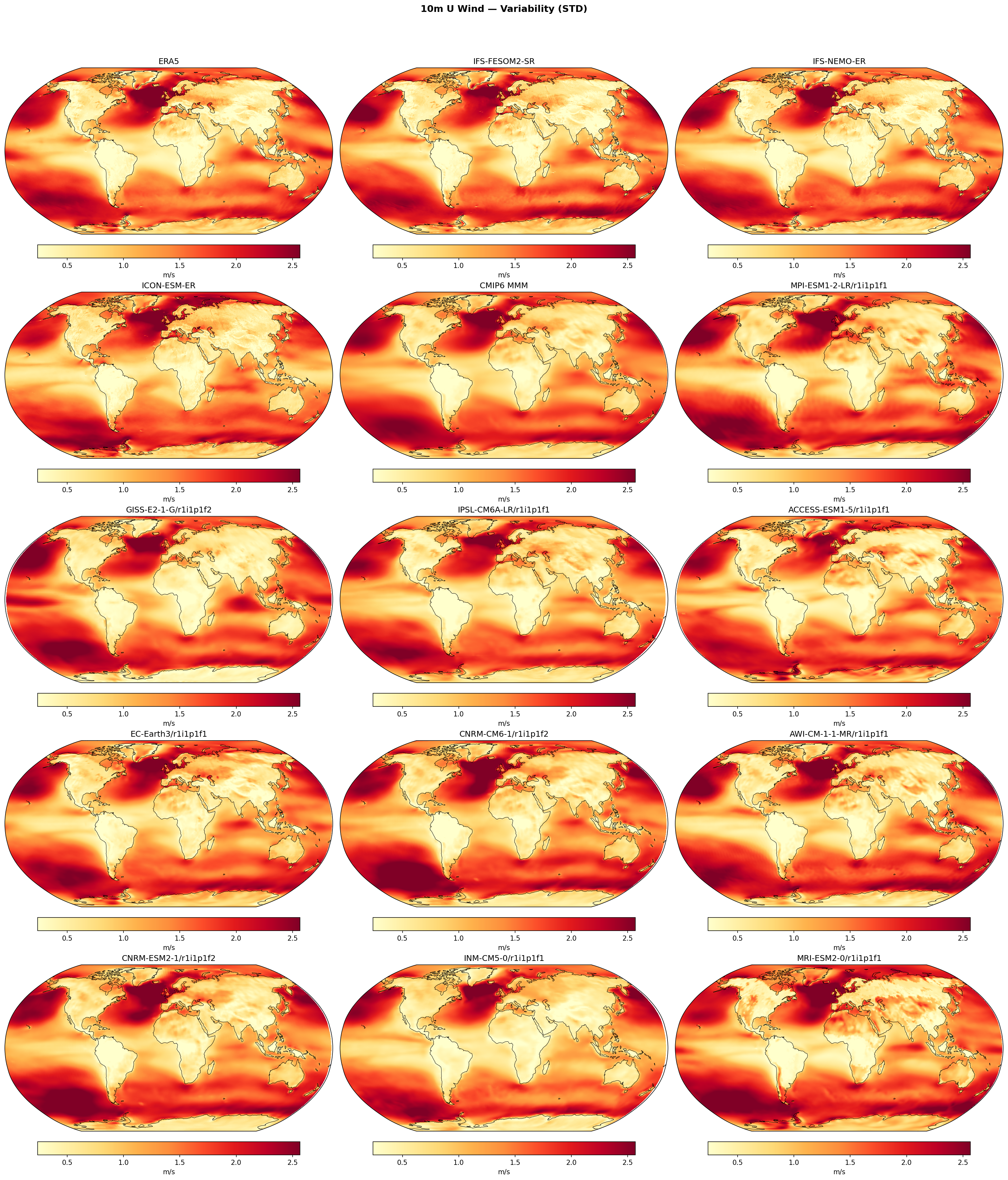
| Variables | uas |
|---|---|
| Models | IFS-FESOM2-SR, IFS-NEMO-ER, ICON-ESM-ER, HadGEM3-GC5, CMIP6 MMM, MPI-ESM1-2-LR/r1i1p1f1, GISS-E2-1-G/r1i1p1f2, IPSL-CM6A-LR/r1i1p1f1, ACCESS-ESM1-5/r1i1p1f1, EC-Earth3/r1i1p1f1, CNRM-CM6-1/r1i1p1f2, AWI-CM-1-1-MR/r1i1p1f1, CNRM-ESM2-1/r1i1p1f2, INM-CM5-0/r1i1p1f1, MRI-ESM2-0/r1i1p1f1 |
| Reference Dataset | ERA5 |
| Units | m/s |
| Period | 1980–2014 |
| IFS-FESOM2-SR | Std Gmean: 1.22 · Diff Gmean: 0.03 · Rmse: 0.19 |
| IFS-NEMO-ER | Std Gmean: 1.20 · Diff Gmean: -0.00 · Rmse: 0.15 |
| ICON-ESM-ER | Std Gmean: 1.21 · Diff Gmean: 0.02 · Rmse: 0.29 |
| HadGEM3-GC5 | Std Gmean: 1.19 · Diff Gmean: -0.00 · Rmse: 0.14 |
| CMIP6 MMM | Std Gmean: 1.27 · Diff Gmean: 0.08 · Rmse: 0.19 |
Summary high
The figure displays the standard deviation of deseasonalised, detrended monthly 10m zonal wind (U-wind), serving as a proxy for low-frequency storm track activity and climate variability. High-resolution EERIE models, particularly HadGEM3-GC5 and IFS-NEMO-ER, show excellent agreement with ERA5, whereas the CMIP6 ensemble tends to overestimate variability magnitudes.
Key Findings
- High variability (>2.0 m/s) is concentrated in the mid-latitude storm tracks of the North Atlantic, North Pacific, and Southern Ocean.
- HadGEM3-GC5 achieves the best performance (RMSE = 0.138 m/s), closely followed by IFS-NEMO-ER (RMSE = 0.145 m/s), both matching ERA5's spatial structure and global mean intensity (~1.19 m/s).
- The CMIP6 Multi-Model Mean and individual CMIP6 models (e.g., CNRM-CM6-1, MRI-ESM2-0) generally exhibit higher variability intensities (CMIP6 MMM global mean = 1.27 m/s) compared to ERA5 and the EERIE simulations.
Spatial Patterns
Variability maxima align with the major storm tracks (40°–60° latitudes), driven by baroclinic instability. Secondary variability features are visible in the tropical Pacific (likely ENSO-related). Land areas consistently show lower variability (<1.0 m/s) due to higher surface roughness/friction compared to the ocean.
Model Agreement
The EERIE models (IFS and HadGEM3 variants) show strong agreement with ERA5, effectively capturing the 'roaring forties' and Northern Hemisphere storm tracks. ICON-ESM-ER has a noticeably higher RMSE (0.286 m/s) than its peers, suggesting some spatial displacement or noise in its variability patterns. Individual CMIP6 models show significant spread, with several overestimating Southern Ocean wind variance.
Physical Interpretation
This metric highlights the intensity of inter-monthly and inter-annual circulation anomalies. The fidelity of the high-resolution models suggests they correctly represent the location and intensity of the jet streams and associated surface westerlies. The positive bias in CMIP6 MMM suggests that coarser resolution models might maintain overly zonal or persistent flow anomalies in the Southern Ocean.
Caveats
- The use of monthly data filters out high-frequency synoptic variance (daily/sub-daily storms); this metric represents lower-frequency variability envelopes.
- Difference maps are not provided, so precise regional sources of the RMSE in ICON-ESM-ER are difficult to diagnose visually.
10m U Wind — Variability Bias (STD diff)
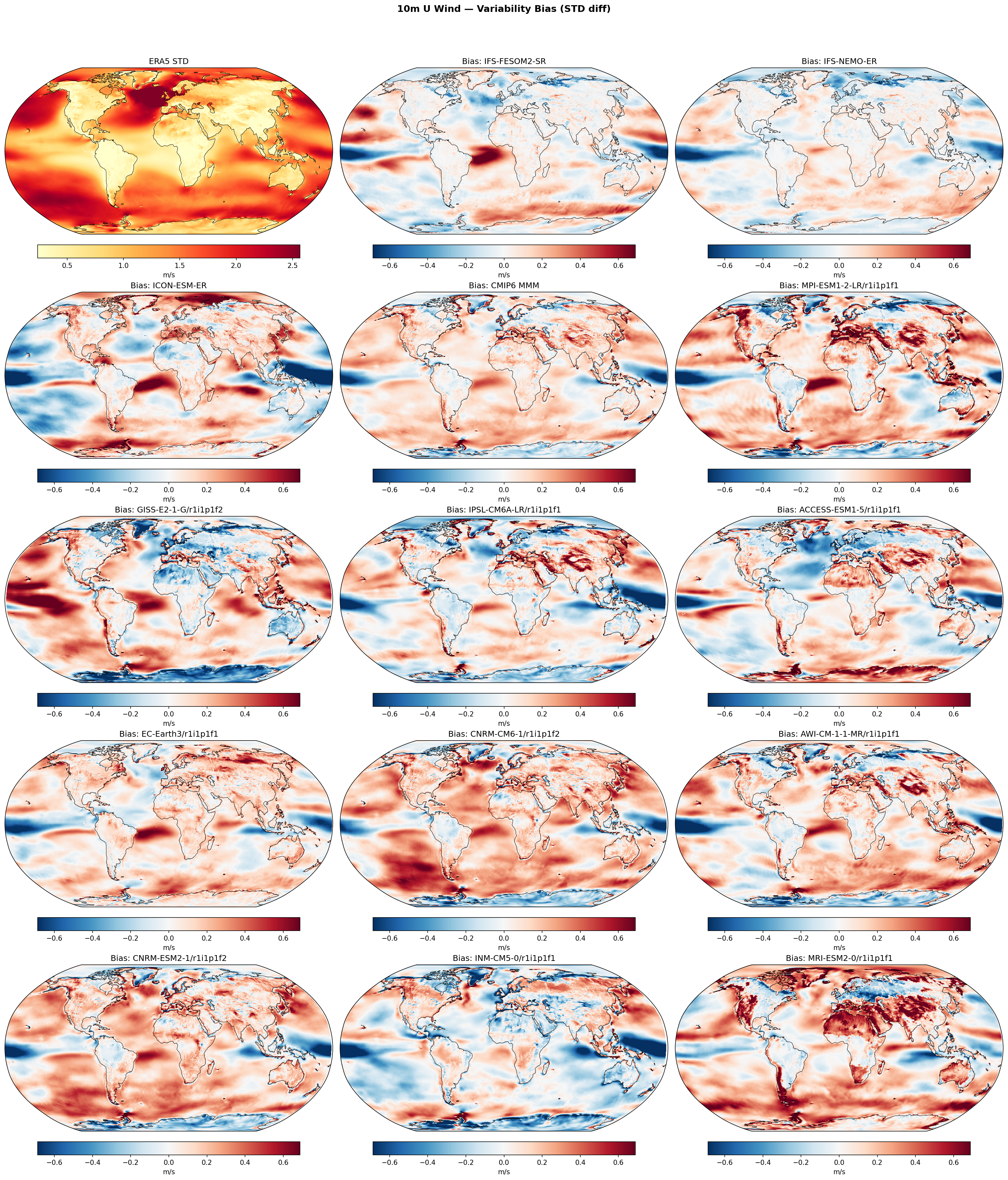
| Variables | uas |
|---|---|
| Models | IFS-FESOM2-SR, IFS-NEMO-ER, ICON-ESM-ER, HadGEM3-GC5, CMIP6 MMM, MPI-ESM1-2-LR/r1i1p1f1, GISS-E2-1-G/r1i1p1f2, IPSL-CM6A-LR/r1i1p1f1, ACCESS-ESM1-5/r1i1p1f1, EC-Earth3/r1i1p1f1, CNRM-CM6-1/r1i1p1f2, AWI-CM-1-1-MR/r1i1p1f1, CNRM-ESM2-1/r1i1p1f2, INM-CM5-0/r1i1p1f1, MRI-ESM2-0/r1i1p1f1 |
| Reference Dataset | ERA5 |
| Units | m/s |
| Period | 1980–2014 |
| IFS-FESOM2-SR | Std Gmean: 1.22 · Diff Gmean: 0.03 · Rmse: 0.19 |
| IFS-NEMO-ER | Std Gmean: 1.20 · Diff Gmean: -0.00 · Rmse: 0.15 |
| ICON-ESM-ER | Std Gmean: 1.21 · Diff Gmean: 0.02 · Rmse: 0.29 |
| HadGEM3-GC5 | Std Gmean: 1.19 · Diff Gmean: -0.00 · Rmse: 0.14 |
| CMIP6 MMM | Std Gmean: 1.27 · Diff Gmean: 0.08 · Rmse: 0.19 |
Summary high
This diagnostic evaluates the standard deviation (variability) of monthly 10m zonal wind (u10) relative to ERA5 reanalysis. The high-resolution EERIE models generally exhibit lower biases and more realistic variability patterns than the CMIP6 Multi-Model Mean and individual CMIP6 members, though distinct regional biases persist in the tropical Pacific and storm tracks.
Key Findings
- HadGEM3-GC5 shows the highest skill, with the lowest RMSE (0.138 m/s) and a lack of strong systematic bias patterns compared to other models.
- IFS variants (NEMO and FESOM) and ICON-ESM-ER share a distinctive bias dipole in the Tropical Pacific (underestimated variability on the equator, overestimated off-equator), indicative of structural errors in ENSO-related wind teleconnections.
- ICON-ESM-ER significantly underestimates wind variability in the North Atlantic storm track and overestimates it in the Southern Ocean, leading to the highest RMSE (0.286 m/s) among the high-resolution group.
- Standard-resolution CMIP6 models (and the MMM) tend to systematically overestimate wind variability (positive bias) over land masses and the tropical oceans, a feature largely improved in the high-resolution simulations.
Spatial Patterns
ERA5 shows peak wind variability in the Southern Ocean and Northern Hemisphere storm tracks. While HadGEM3-GC5 captures these magnitudes well, IFS-FESOM2-SR and ICON-ESM-ER show excessive variability (red bias) in the Southern Ocean. In the tropics, the IFS and ICON models exhibit a zonal banding structure in biases (negative equator, positive subtropics) not seen in HadGEM3. CMIP6 models frequently display strong positive variability biases over continents (e.g., MRI-ESM2-0, GISS-E2-1-G).
Model Agreement
HadGEM3-GC5 and IFS-NEMO-ER agree best with observations (lowest RMSEs). There is notable divergence in the North Atlantic, where ICON underestimates variability while others are neutral or slightly negative. The EERIE models as a group outperform the CMIP6 ensemble, which generally suffers from excessive variability.
Physical Interpretation
The patterns of variability are driven by mid-latitude cyclone activity (storm tracks) and tropical coupled modes (ENSO). The tropical bias dipoles in IFS/ICON suggest the atmospheric response to ENSO SST anomalies is too meridionally confined or meridionally shifted. The reduction in excessive land-based variability in high-resolution models suggests that improved orography resolution and surface drag parameterizations likely dampen unrealistic surface wind fluctuations found in coarser CMIP6 models.
Caveats
- ERA5 winds are a model product (IFS-based), which might influence comparisons, although the non-IFS HadGEM3 model actually performs best here.
- The analysis considers monthly variability, so it captures sub-seasonal to interannual variance but filters out high-frequency synoptic weather events.
10m V Wind — Variability (STD)
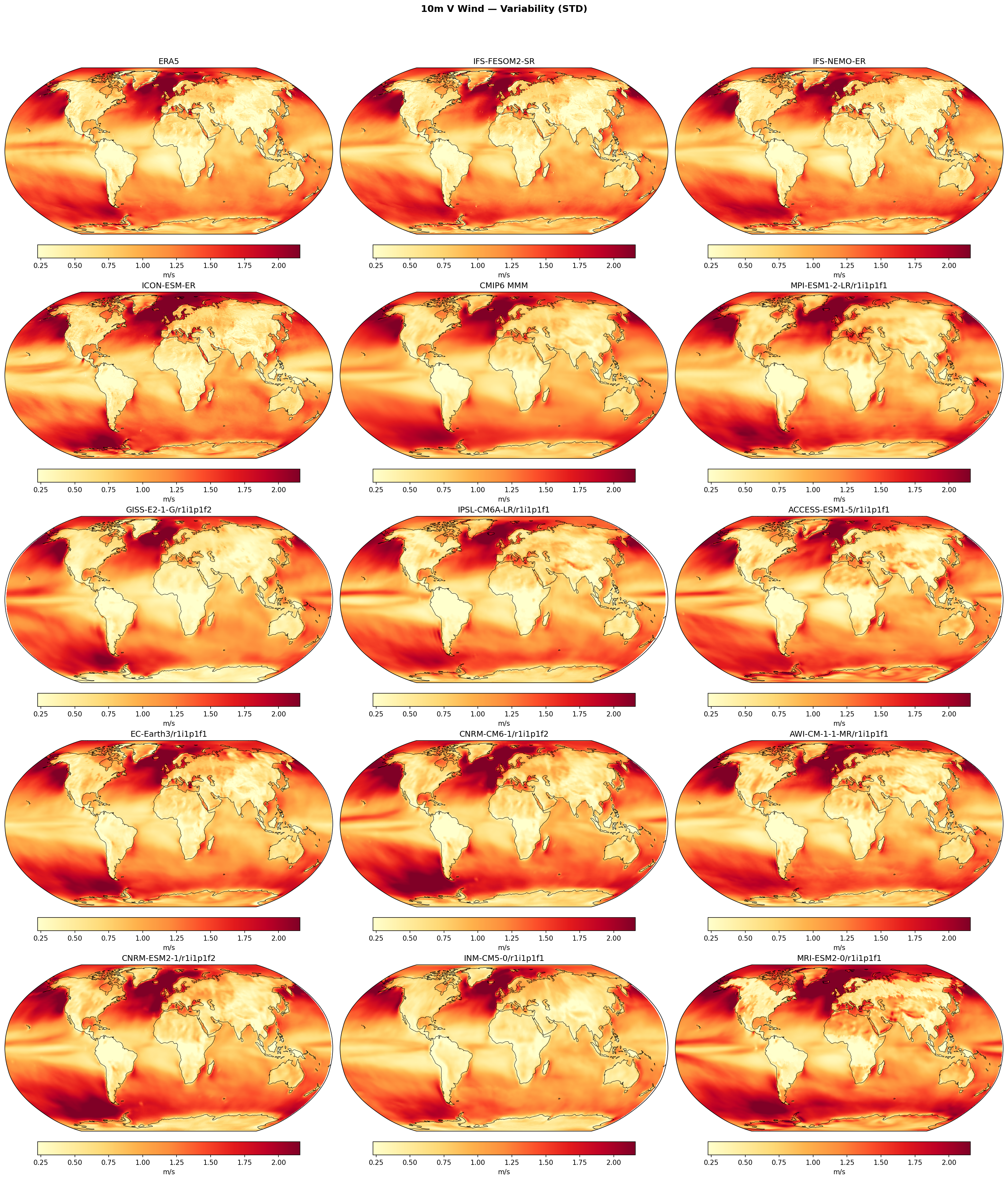
| Variables | vas |
|---|---|
| Models | IFS-FESOM2-SR, IFS-NEMO-ER, ICON-ESM-ER, HadGEM3-GC5, CMIP6 MMM, MPI-ESM1-2-LR/r1i1p1f1, GISS-E2-1-G/r1i1p1f2, IPSL-CM6A-LR/r1i1p1f1, ACCESS-ESM1-5/r1i1p1f1, EC-Earth3/r1i1p1f1, CNRM-CM6-1/r1i1p1f2, AWI-CM-1-1-MR/r1i1p1f1, CNRM-ESM2-1/r1i1p1f2, INM-CM5-0/r1i1p1f1, MRI-ESM2-0/r1i1p1f1 |
| Reference Dataset | ERA5 |
| Units | m/s |
| Period | 1980–2014 |
| IFS-FESOM2-SR | Std Gmean: 0.95 · Diff Gmean: 0.02 · Rmse: 0.12 |
| IFS-NEMO-ER | Std Gmean: 0.94 · Diff Gmean: 0.00 · Rmse: 0.10 |
| ICON-ESM-ER | Std Gmean: 0.99 · Diff Gmean: 0.05 · Rmse: 0.19 |
| HadGEM3-GC5 | Std Gmean: 0.97 · Diff Gmean: 0.03 · Rmse: 0.12 |
| CMIP6 MMM | Std Gmean: 1.01 · Diff Gmean: 0.07 · Rmse: 0.15 |
Summary high
This figure displays the global spatial distribution of climate variability for 10m meridional wind (V), quantified as the standard deviation of deseasonalised and detrended monthly anomalies from 1980–2014.
Key Findings
- The IFS-NEMO-ER and IFS-FESOM2-SR models show the best agreement with ERA5, exhibiting the lowest RMSE values (~0.10–0.12 m/s) and accurately capturing the intensity of variability in major storm tracks.
- ICON-ESM-ER systematically overestimates wind variability compared to ERA5 (RMSE ~0.19 m/s), with excessive standard deviation evident in the Southern Ocean and North Pacific.
- The CMIP6 Multi-Model Mean (MMM) captures the broad spatial structure but lacks the fine-scale definition of the high-resolution models; however, individual CMIP6 models show large spread, with some (e.g., MRI-ESM2-0) showing intense tropical variability and others (e.g., GISS-E2-1-G) appearing damped.
- HadGEM3-GC5 performs well (RMSE ~0.12 m/s) but shows slightly elevated variability in the tropical Pacific relative to ERA5.
Spatial Patterns
Dominant variability (>1.75 m/s) is located in the major mid-latitude storm tracks: the Southern Ocean (40–60°S), North Atlantic, and North Pacific. A secondary band of high variability exists in the tropical Pacific, associated with the Intertropical Convergence Zone (ITCZ) and ENSO dynamics. Variability is generally lower over land and in the subtropical high-pressure belts.
Model Agreement
There is strong inter-model agreement on the location of maximum variability (storm tracks). The primary divergence is in amplitude: IFS variants match ERA5 closely, while ICON-ESM-ER and some CMIP6 members predict significantly more energetic low-frequency wind variability.
Physical Interpretation
The patterns reflect the interannual and intra-seasonal modulation of the general circulation. High variability in the mid-latitudes corresponds to the shifting position and intensity of storm tracks (influenced by modes like the NAO and SAM). In the tropics, variability is driven by shifts in trade wind convergence and monsoonal flows, strongly linked to ENSO cycles.
Caveats
- The analysis uses monthly data, meaning this variability represents low-frequency shifts in circulation patterns rather than high-frequency synoptic storminess (which would require daily data).
- CMIP6 MMM smoothness is an artifact of ensemble averaging, masking the diversity of biases in individual low-resolution models.
10m V Wind — Variability Bias (STD diff)
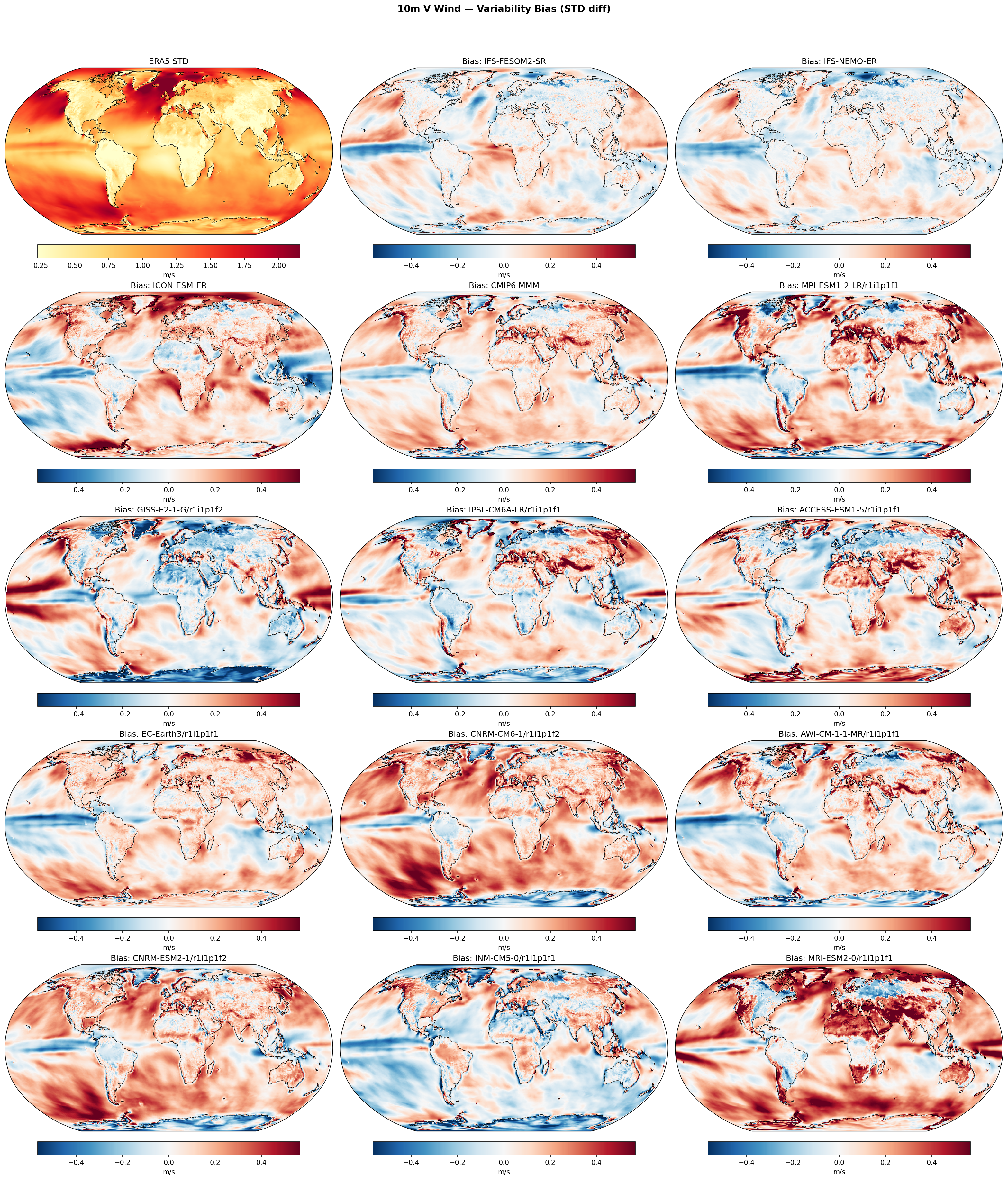
| Variables | vas |
|---|---|
| Models | IFS-FESOM2-SR, IFS-NEMO-ER, ICON-ESM-ER, HadGEM3-GC5, CMIP6 MMM, MPI-ESM1-2-LR/r1i1p1f1, GISS-E2-1-G/r1i1p1f2, IPSL-CM6A-LR/r1i1p1f1, ACCESS-ESM1-5/r1i1p1f1, EC-Earth3/r1i1p1f1, CNRM-CM6-1/r1i1p1f2, AWI-CM-1-1-MR/r1i1p1f1, CNRM-ESM2-1/r1i1p1f2, INM-CM5-0/r1i1p1f1, MRI-ESM2-0/r1i1p1f1 |
| Reference Dataset | ERA5 |
| Units | m/s |
| Period | 1980–2014 |
| IFS-FESOM2-SR | Std Gmean: 0.95 · Diff Gmean: 0.02 · Rmse: 0.12 |
| IFS-NEMO-ER | Std Gmean: 0.94 · Diff Gmean: 0.00 · Rmse: 0.10 |
| ICON-ESM-ER | Std Gmean: 0.99 · Diff Gmean: 0.05 · Rmse: 0.19 |
| HadGEM3-GC5 | Std Gmean: 0.97 · Diff Gmean: 0.03 · Rmse: 0.12 |
| CMIP6 MMM | Std Gmean: 1.01 · Diff Gmean: 0.07 · Rmse: 0.15 |
Summary high
Diagnostic maps showing the bias in the standard deviation of 10m meridional wind (v-component) for EERIE high-resolution models and CMIP6 models relative to ERA5. The high-resolution EERIE models significantly outperform standard CMIP6 models, which exhibit widespread systematic overestimation of wind variability.
Key Findings
- IFS-NEMO-ER and IFS-FESOM2-SR display exceptional skill (RMSE ~0.10-0.12 m/s), showing primarily neutral biases with only slight underestimation in storm tracks.
- CMIP6 models (MMM and individuals like GISS-E2-1-G, CNRM-CM6-1) systematically overestimate wind variability (positive bias) over land masses and tropical oceans.
- ICON-ESM-ER diverges from the IFS group with higher variability (positive bias) in the Southern Ocean and distinct negative biases in the eastern tropical Pacific.
Spatial Patterns
ERA5 shows peak variability in the mid-latitude storm tracks (>1.75 m/s). CMIP6 models consistently show strong positive biases (excess variability) over continents and the Indo-Pacific warm pool. In contrast, EERIE models largely eliminate the continental bias. ICON-ESM-ER and several CMIP6 models show enhanced variability in the Southern Ocean, whereas IFS variants show slight negative biases there.
Model Agreement
There is high agreement between the two IFS-based simulations (NEMO vs FESOM), suggesting the atmospheric component dictates this metric. EERIE models generally agree on reducing the gross positive biases seen in the CMIP6 ensemble, though ICON is an outlier among the high-res group.
Physical Interpretation
The widespread excess variability over land in coarser CMIP6 models suggests issues with surface drag parameterisations or unresolved orography which are improved at higher resolutions. In the tropics, the positive bias in CMIP6 likely stems from convective parameterisations generating excessive intermittency or grid-scale noise, which appears better constrained in the high-resolution EERIE simulations.
Caveats
- ERA5 reanalysis relies on an IFS-based model, potentially biasing comparisons in favour of IFS-FESOM/NEMO in data-sparse regions like the Southern Ocean.
- The analysis focuses on variability magnitude (STD) and does not assess the temporal phasing or spectral characteristics of the variability.