Ocean 3d Ocean Evaluation (EN4)
Synthesis
Related diagnostics
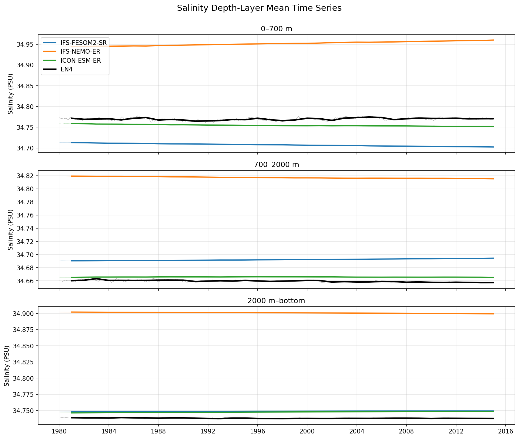
Salinity Depth-Layer Time Series
| Variables | thetao, so |
|---|---|
| Models | IFS-FESOM2-SR, IFS-NEMO-ER, ICON-ESM-ER, HadGEM3-GC5, EN4 |
| Reference Dataset | EN4 v4.2.2 |
| Units | K |
| Period | 1980–2014 |
Summary high
Time series of global volume-weighted mean salinity in three depth layers (0–700 m, 700–2000 m, >2000 m) for 1980–2014, comparing four coupled models against EN4 analysis. The models exhibit significant biases and persistent linear drifts indicative of equilibration processes, with marked divergence in the upper ocean.
Key Findings
- HadGEM3-GC5 shows a severe fresh bias (~0.13 PSU) in the upper ocean (0–700 m) but a saline bias in the deep ocean (>2000 m), suggesting a strong stratification error.
- IFS-FESOM2-SR exhibits a continuous freshening drift in the upper ocean and a salinification drift in the deep ocean, consistent with a vertical redistribution of salt.
- IFS-NEMO-ER displays the opposite tendency to other models in the deep ocean, with a distinct freshening drift below 700 m and slight salinification at the surface.
- Models capture negligible interannual variability compared to EN4 observations, with time evolution dominated by monotonic drifts from initialization.
Spatial Patterns
Biases are vertically structured: HadGEM3-GC5 and IFS-FESOM2-SR are fresh at the surface and salty at depth (stabilising bias), whereas IFS-NEMO-ER is closer to observations at the surface but fresh at depth. The spread between models is largest in the upper ocean (~0.15 PSU range) and tightens in the deep ocean (~0.04 PSU range), though deep trends are persistent.
Model Agreement
Inter-model agreement is poor regarding absolute magnitude, particularly in the upper ocean. Trends also diverge, with some models freshening and others salinifying in the same layers. ICON-ESM-ER generally shows the smallest drifts and biases in the intermediate layer (700–2000 m).
Physical Interpretation
The linear drifts indicate that the models have not reached equilibrium and are adjusting from their initial states (likely EN4-based). The 'fresh surface / salty deep' pattern in HadGEM3-GC5 and IFS-FESOM2-SR suggests issues with vertical mixing or surface freshwater flux imbalances (e.g., precipitation or runoff spread) that prevent adequate ventilation of deep salt. IFS-NEMO-ER's deep freshening implies a different mechanism, possibly excessive ventilation or initial adjustment shocks.
Caveats
- The analysis period (1980–2014) is short relative to deep ocean mixing timescales, so trends largely represent model spin-up drift.
- EN4 deep ocean data relies on sparse observations, particularly before the Argo era (pre-2000s), increasing observational uncertainty in the bottom panel.
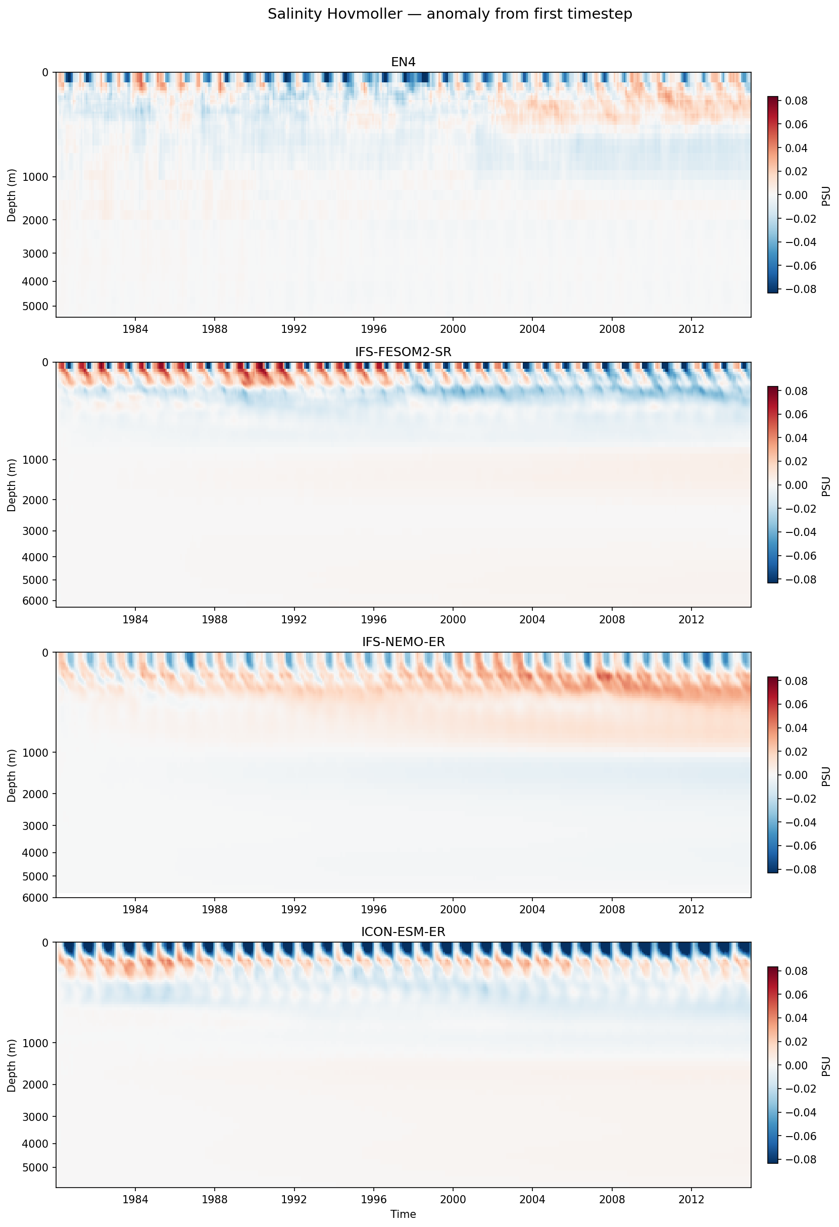
Salinity Hovmoller (first-timestep anomaly)
| Variables | thetao, so |
|---|---|
| Models | IFS-FESOM2-SR, IFS-NEMO-ER, ICON-ESM-ER, HadGEM3-GC5 |
| Reference Dataset | EN4 v4.2.2 |
| Units | K |
| Period | 1980–2014 |
Summary high
This time-depth Hovmoller diagram compares the evolution of global-mean salinity anomalies (relative to the first timestep) in the upper 6000m of the ocean across four high-resolution coupled models and EN4 observations from 1980 to 2014.
Key Findings
- IFS-NEMO-ER exhibits a strong, monotonic salinification drift (positive anomaly >0.04 PSU) dominating the upper 1500m, significantly exceeding observational variability.
- In contrast, ICON-ESM-ER and IFS-FESOM2-SR show a persistent subsurface freshening drift (negative anomaly) centered between 200m and 800m depth.
- HadGEM3-GC5 displays a marked vertical dipole drift: strong salinification in the surface layer (0–300m) and freshening in the intermediate layers (500–1500m).
- EN4 observations show high stability below the surface mixed layer, with anomalies generally smaller than ±0.02 PSU, indicating that the strong trends in all models represent significant drifts.
Spatial Patterns
Model drifts are primarily confined to the upper 2000m, with the deep ocean (>3000m) remaining stable in all simulations. The surface layers in all panels capture the seasonal cycle, but the multi-decadal drifts in the thermocline and intermediate waters dominate the model signals.
Model Agreement
There is low inter-model agreement regarding the sign and vertical structure of salinity drift. Even models sharing the same atmospheric component (IFS-FESOM2-SR and IFS-NEMO-ER) show opposite subsurface tendencies (freshening vs. salinification), isolating the ocean model formulation (FESOM vs. NEMO) as a key driver of uncertainty.
Physical Interpretation
The drifts likely result from imbalances in the surface freshwater budget (P-E) or deficiencies in vertical mixing and ventilation processes. The subsurface freshening in ICON and FESOM suggests issues with mode water formation or subduction of fresh anomalies, while the strong salinification in IFS-NEMO-ER suggests excessive evaporation or vigorous vertical mixing bringing salt upwards. The HadGEM3 dipole implies a stratification change, potentially due to surface flux mismatches.
Caveats
- Global mean averaging obscures regional cancellations (e.g., Atlantic salinification vs. Pacific freshening).
- Anomalies relative to the first timestep conflate intrinsic model drift (spin-up) with forced climate trends, although the divergence from EN4 suggests drift is the dominant factor.
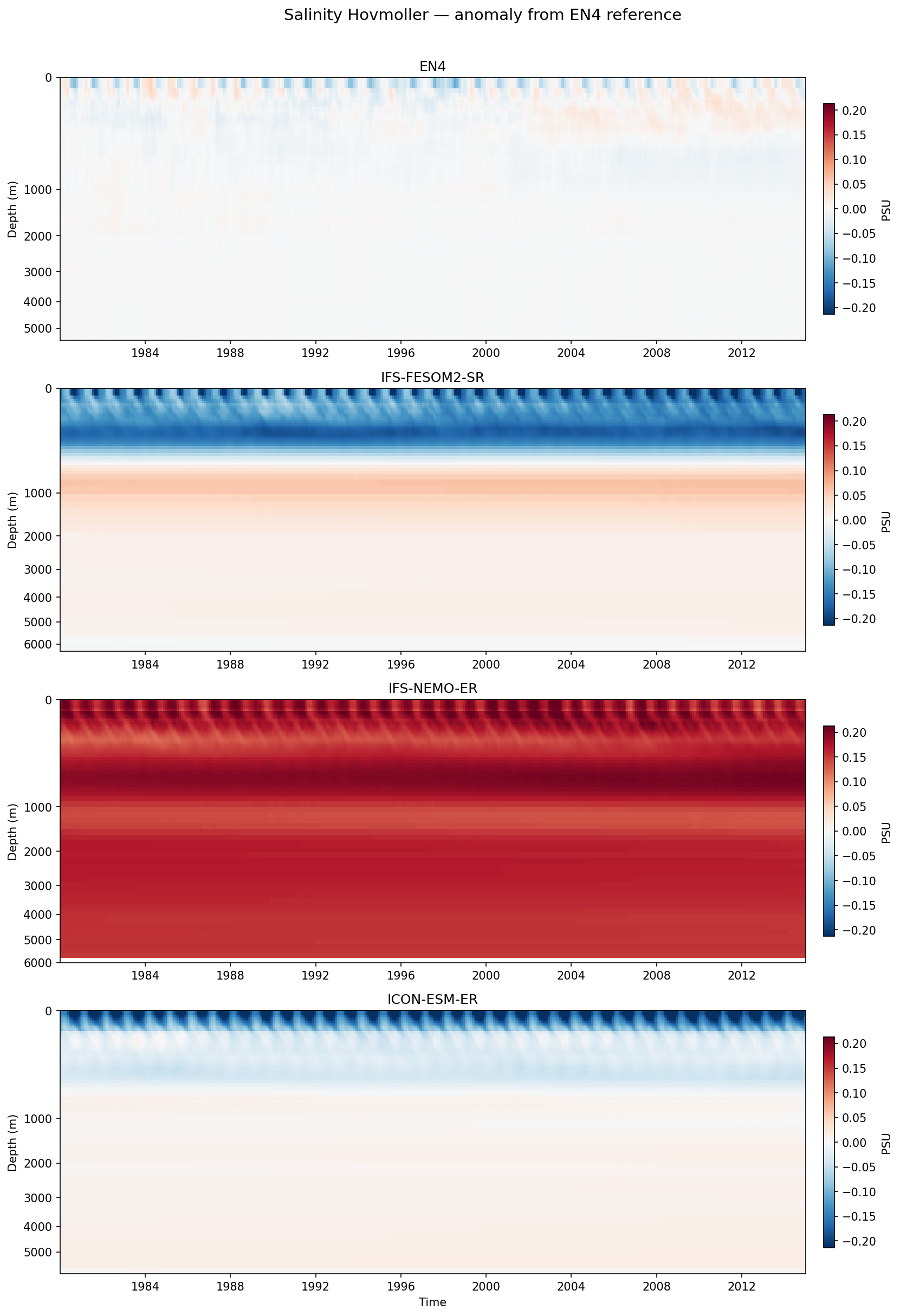
Salinity Hovmoller (EN4-ref anomaly)
| Variables | thetao, so |
|---|---|
| Models | IFS-FESOM2-SR, IFS-NEMO-ER, ICON-ESM-ER, HadGEM3-GC5 |
| Reference Dataset | EN4 v4.2.2 |
| Units | K |
| Period | 1980–2014 |
Summary high
This Hovmoller diagram illustrates the time-depth evolution of global-mean salinity anomalies (drift) relative to the EN4 initial reference profile from 1980 to 2014. While the observational baseline (EN4) and IFS-NEMO-ER remain relatively stable, other models exhibit significant drifts, predominantly characterized by strong upper-ocean freshening.
Key Findings
- IFS-NEMO-ER performs best, showing minimal salinity drift across the entire depth range, closely tracking the stability of the EN4 observational reference.
- HadGEM3-GC5 and IFS-FESOM2-SR exhibit a pronounced dipole bias structure: severe freshening in the upper 800 m (exceeding -0.20 PSU) and compensatory salinification at intermediate depths (800–3000 m).
- ICON-ESM-ER displays strong surface freshening in the top 500 m, similar to IFS-FESOM2-SR but with less pronounced drift in the deep ocean.
Spatial Patterns
The dominant pattern in the drifting models (HadGEM3, IFS-FESOM2, ICON) is a stratification-enhancing bias: fresh anomalies accumulate in the upper ocean while intermediate/deep layers either remain stable or become saltier. This drift is established early in the simulation (first 5-10 years) and persists.
Model Agreement
There is significant divergence in model fidelity. IFS-NEMO-ER stands out for its stability, whereas IFS-FESOM2-SR, ICON-ESM-ER, and HadGEM3-GC5 all agree on a tendency towards upper-ocean freshening, though magnitudes differ.
Physical Interpretation
The widespread surface freshening suggests a common systemic issue, potentially related to excessive precipitation (e.g., double ITCZ biases), insufficient surface evaporation, or weak vertical mixing which traps fresh water at the surface. The intermediate salinification in HadGEM3 and IFS-FESOM2 may indicate issues with water mass ventilation (e.g., NADW formation) or a readjustment of the thermohaline structure from the initialized state.
Caveats
- Global averaging obscures regional patterns; surface freshening may be dominated by specific basins (e.g., Arctic or North Atlantic).
- The reference is fixed to the start of the period (implied by the EN4 panel showing minimal change), so the figure visualizes model drift from initialization rather than just bias against concurrent observations.
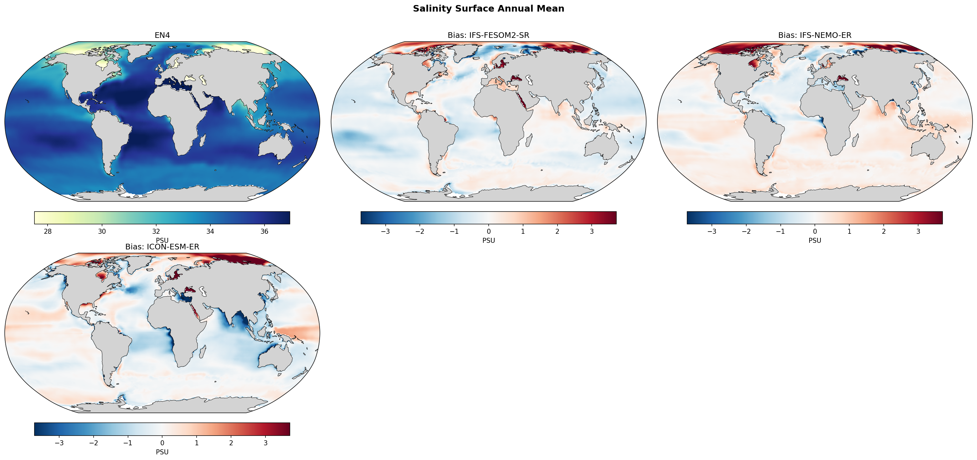
Salinity Surface Annual Mean Bias
| Variables | thetao, so |
|---|---|
| Models | IFS-FESOM2-SR, IFS-NEMO-ER, ICON-ESM-ER, HadGEM3-GC5 |
| Reference Dataset | EN4 v4.2.2 |
| Units | K |
| Period | 1980–2014 |
| IFS-FESOM2-SR | Global Mean Bias: -0.18 · Rmse: 0.69 |
| IFS-NEMO-ER | Global Mean Bias: -0.00 · Rmse: 0.71 |
| ICON-ESM-ER | Global Mean Bias: -0.19 · Rmse: 1.19 |
| HadGEM3-GC5 | Global Mean Bias: -0.16 · Rmse: 0.77 |
Summary high
This figure evaluates annual mean sea surface salinity (SSS) biases in four high-resolution coupled models against EN4 observations. While all models share a systematic strong positive bias in the Arctic, they diverge significantly in the tropics, with ICON-ESM-ER exhibiting severe fresh biases in the Indo-Pacific that drive its root-mean-square error (RMSE) well above the others.
Key Findings
- All models exhibit a prominent positive salinity bias (>2 PSU) in the central Arctic Ocean, indicating a common failure to preserve the surface halocline or adequately retain freshwater.
- ICON-ESM-ER shows the highest RMSE (1.19 PSU) and a distinct, intense fresh bias throughout the Bay of Bengal, Arabian Sea, and broader Indian Ocean, likely linked to excessive precipitation or river runoff handling.
- IFS-FESOM2-SR and IFS-NEMO-ER perform best globally (RMSE ~0.7 PSU), though IFS-NEMO-ER has a near-zero global mean bias (-0.004 PSU) compared to the slight fresh bias in FESOM (-0.18 PSU).
- HadGEM3-GC5 displays distinct fresh biases along eastern boundary upwelling zones (Peru-Chile, Benguela, California currents), suggesting issues with subsurface water properties or local surface fluxes.
Spatial Patterns
The Arctic and semi-enclosed seas (Mediterranean, Red Sea, Baltic) consistently show strong positive (salty) biases across all simulations. In contrast, the tropical oceans show model-specific behavior: IFS models are generally closer to observations with patchy fresh biases in the ITCZ regions; ICON is dominated by a vast fresh signal in the Asian monsoon region; and HadGEM3 shows coastal freshening in upwelling regions. Sharp bias dipoles near major river mouths (Amazon, Congo) highlight challenges in resolving plume advection.
Model Agreement
Models agree on high-latitude salinification (Arctic) and salinification of marginal seas (Mediterranean). They disagree strongly in the Indian Ocean (ICON outlier) and eastern boundary currents (HadGEM3 outlier).
Physical Interpretation
The pervasive Arctic salty bias suggests excessive vertical mixing bringing salty Atlantic water to the surface, or insufficient sea ice meltwater/river runoff stratification. The positive bias in the Mediterranean likely results from restricted exchange through the Strait of Gibraltar or evaporation-precipitation imbalances. ICON's Indian Ocean fresh bias is likely coupled to an intense precipitation bias (wet bias) typical of some models in the monsoon region. HadGEM3's coastal fresh biases may result from upwelling of fresher-than-observed subsurface waters or errors in coastal cloud/precip processes.
Caveats
- Observational coverage in the Arctic (EN4) is sparser than in lower latitudes, increasing uncertainty in the high-latitude bias assessment.
- Coastal biases near major river outflows may be sensitive to the specific river routing and discharge datasets used by each model.
Salinity Surface DJF Bias

| Variables | thetao, so |
|---|---|
| Models | IFS-FESOM2-SR, IFS-NEMO-ER, ICON-ESM-ER, HadGEM3-GC5 |
| Reference Dataset | EN4 v4.2.2 |
| Units | K |
| Period | 1980–2014 |
| IFS-FESOM2-SR | Global Mean Bias: -0.18 · Rmse: 0.77 |
| IFS-NEMO-ER | Global Mean Bias: -0.01 · Rmse: 0.72 |
| ICON-ESM-ER | Global Mean Bias: -0.18 · Rmse: 1.19 |
| HadGEM3-GC5 | Global Mean Bias: -0.17 · Rmse: 0.79 |
Summary high
This figure displays DJF surface salinity biases relative to EN4 observations, revealing a systematic salty bias in the central Arctic across all models and divergent behaviors in the North Atlantic and Tropics.
Key Findings
- All four models exhibit a strong positive (salty) bias in the Central Arctic and Canadian Archipelago, exceeding +3 PSU in some regions.
- IFS-NEMO-ER demonstrates the best performance with the lowest RMSE (0.72 PSU) and a negligible global mean bias (-0.01 PSU), whereas ICON-ESM-ER has the highest RMSE (1.19 PSU).
- A prominent fresh bias characterizes the North Atlantic subpolar gyre and Gulf Stream extension in ICON-ESM-ER, HadGEM3-GC5, and IFS-FESOM2-SR, contrasting with IFS-NEMO-ER's more neutral or slightly salty bias in this region.
Spatial Patterns
The Central Arctic is uniformly too salty. In the North Atlantic, a 'fresh blob' south of Greenland is evident in most models, most severe in ICON. The Tropical Pacific shows distinct inter-model differences: IFS-NEMO-ER has a strong salty bias in the cold tongue/eastern Pacific, while IFS-FESOM2-SR and HadGEM3-GC5 tend to be fresher in the central/western basin. ICON-ESM-ER shows unique strong biases in the Indian Ocean (fresh Bay of Bengal, salty Arabian Sea). The Mediterranean is consistently too salty in biases.
Model Agreement
Models strongly agree on the positive bias in the high Arctic. They disagree significantly in the Tropical Pacific and North Atlantic current regions. IFS-FESOM2-SR and HadGEM3-GC5 show the strongest spatial similarity in their bias patterns (fresh Southern Ocean, fresh North Atlantic, salty Tropical Atlantic).
Physical Interpretation
The Arctic salty bias suggests issues with freshwater storage (Beaufort Gyre) or vertical mixing of brine rejection during sea ice formation. The North Atlantic fresh biases likely reflect a too-zonal North Atlantic Current or weak salt transport into the subpolar gyre, a common bias often linked to SST cold biases. Tropical biases (e.g., salty Tropical Atlantic) likely stem from Precipitation minus Evaporation (P-E) errors, such as a displaced ITCZ or underestimated Amazon runoff (visible as localized salty spots near river mouths in FESOM/HadGEM3).
Caveats
- Metadata incorrectly lists units as 'K'; the actual unit is PSU.
- Surface salinity is highly sensitive to precipitation biases, making it difficult to separate ocean dynamics errors from atmospheric forcing errors.
Salinity Surface JJA Bias
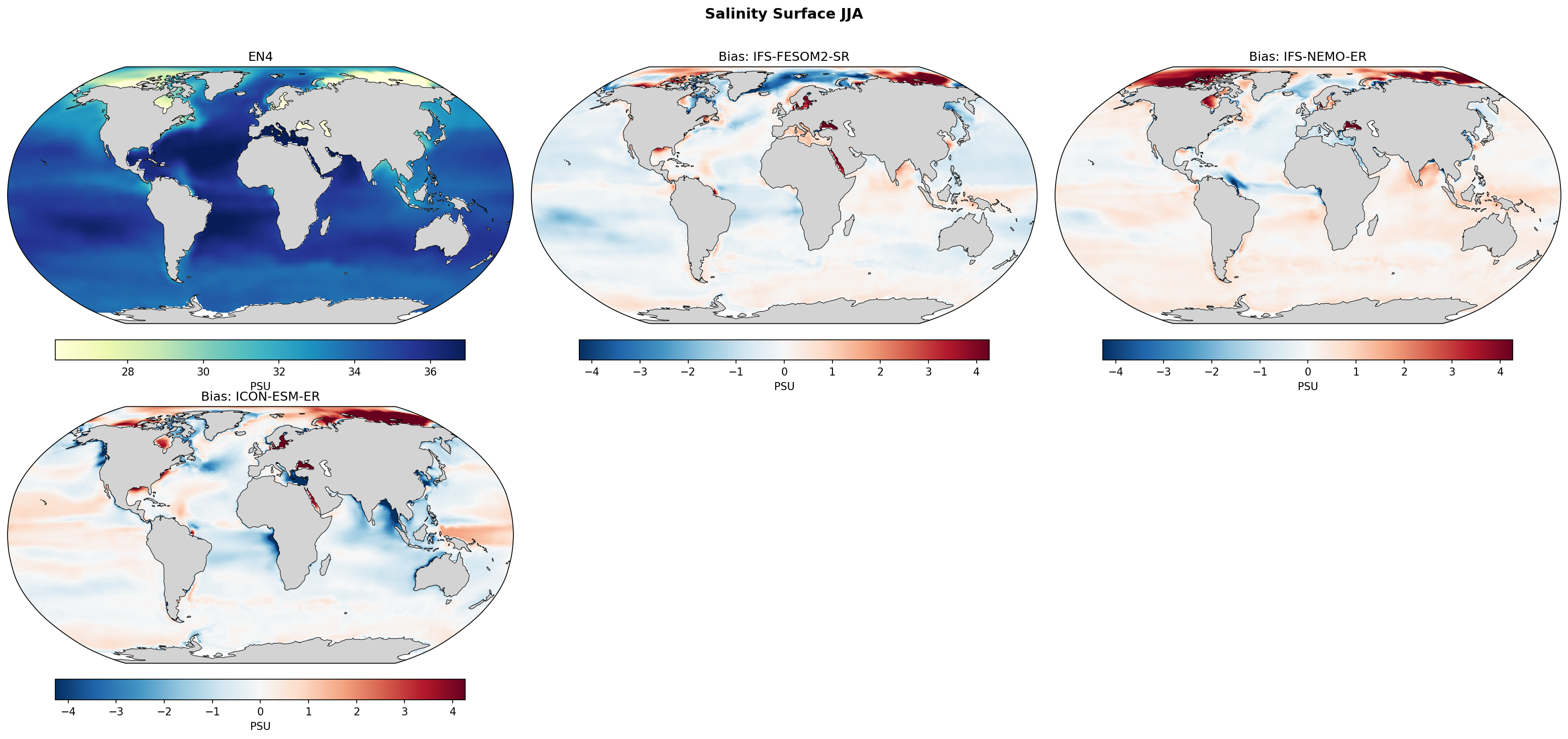
| Variables | thetao, so |
|---|---|
| Models | IFS-FESOM2-SR, IFS-NEMO-ER, ICON-ESM-ER, HadGEM3-GC5 |
| Reference Dataset | EN4 v4.2.2 |
| Units | K |
| Period | 1980–2014 |
| IFS-FESOM2-SR | Global Mean Bias: -0.19 · Rmse: 0.77 |
| IFS-NEMO-ER | Global Mean Bias: 0.02 · Rmse: 0.82 |
| ICON-ESM-ER | Global Mean Bias: -0.20 · Rmse: 1.29 |
| HadGEM3-GC5 | Global Mean Bias: -0.14 · Rmse: 0.85 |
Summary high
This figure evaluates June-August (JJA) sea surface salinity (SSS) biases in four high-resolution coupled models relative to EN4 v4.2.2 observations. While models capture the broad zonal SSS structures, significant regional biases exist, particularly in the Arctic and major river outflow regions.
Key Findings
- All models exhibit a prominent positive (salty) bias in the Arctic Ocean, particularly along the Eurasian shelf, with ICON-ESM-ER and IFS-NEMO-ER showing the most severe Arctic salinification (>4 PSU).
- A negative (fresh) bias dominates the North Atlantic subpolar gyre in ICON-ESM-ER, HadGEM3-GC5, and IFS-FESOM2-SR, likely associated with circulation path errors or freshwater export from the Arctic.
- Major river plumes (Amazon, Congo) consistently show positive (salty) biases near the coast (dark red patches), suggesting underestimated runoff volumes or excessive mixing of fresh water in the models.
- ICON-ESM-ER has the highest global RMSE (1.29 PSU), driven by strong widespread fresh biases in the Indian Ocean, West Pacific, and North Atlantic, contrasting with its strong salty bias in the Arctic.
- IFS-FESOM2-SR achieves the lowest RMSE (0.77 PSU), showing the most balanced performance globally, though it shares the common Arctic and Mediterranean salty biases.
Spatial Patterns
The most striking spatial pattern is the contrast between high-latitude biases: distinct salinification in the Arctic versus freshening in the North Atlantic subpolar region (in 3 of 4 models). The Mediterranean Sea is consistently too salty across most models. In the tropics, biases are often localized near river mouths or follow zonal precipitation bands, with ICON showing a unique basin-wide freshening in the Indian Ocean.
Model Agreement
Models agree on the sign of biases in the Arctic (salty) and near major river mouths (salty). There is divergence in the North Atlantic, where IFS-NEMO-ER shows a mixed/salty signal while others are fresh. Inter-model spread is largest in the Indian Ocean, where ICON is a fresh outlier compared to the others.
Physical Interpretation
The pervasive Arctic salty bias suggests issues with sea ice meltwater distribution, river runoff parameterization, or excessive Atlantic water inflow. The salty biases at river mouths (Amazon, Congo) indicate that despite high resolution, models struggle to maintain fresh surface plumes against mixing or lack sufficient discharge forcing. The fresh bias in the North Atlantic subpolar gyre, common in climate models, is often linked to the 'cold blob' phenomenon and weak northward heat/salt transport by the AMOC or gyre circulation errors.
Caveats
- EN4 observational data in the Arctic has higher uncertainty due to sparse sampling.
- JJA is a season of high river runoff and ice melt; biases here may reflect seasonal cycle errors rather than annual mean states.
Temperature Surface Annual Mean Bias
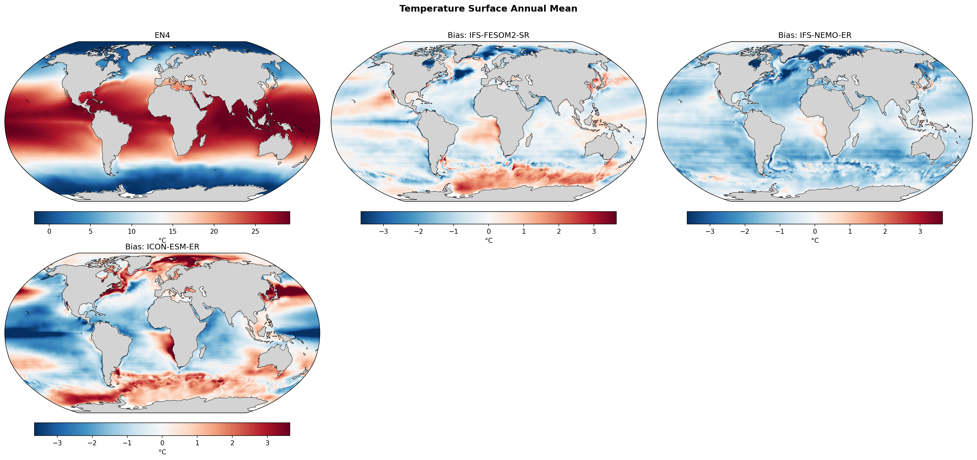
| Variables | thetao, so |
|---|---|
| Models | IFS-FESOM2-SR, IFS-NEMO-ER, ICON-ESM-ER, HadGEM3-GC5 |
| Reference Dataset | EN4 v4.2.2 |
| Units | K |
| Period | 1980–2014 |
| IFS-FESOM2-SR | Global Mean Bias: -0.19 · Rmse: 0.91 |
| IFS-NEMO-ER | Global Mean Bias: -1.05 · Rmse: 1.29 |
| ICON-ESM-ER | Global Mean Bias: -0.36 · Rmse: 1.70 |
| HadGEM3-GC5 | Global Mean Bias: 0.32 · Rmse: 0.84 |
Summary high
This figure compares annual mean Sea Surface Temperature (SST) biases against EN4 observations for four high-resolution coupled models. While HadGEM3-GC5 achieves the lowest spatial error (RMSE 0.84 K), the models exhibit divergent mean states, ranging from a severe systematic cold bias in IFS-NEMO-ER to strong regional contrasts in ICON-ESM-ER.
Key Findings
- IFS-NEMO-ER exhibits a pervasive, systematic global cold bias (mean -1.05 K), significantly colder than the other models.
- ICON-ESM-ER displays the highest spatial variability (RMSE 1.70 K) with intense warm biases (>3 K) in Western Boundary Current extensions (Gulf Stream, Kuroshio) and the South Atlantic, contrasting with cold biases in the tropical Pacific.
- HadGEM3-GC5 performs best statistically (RMSE 0.84 K) but shows characteristic warm biases in Eastern Boundary Upwelling Systems (e.g., Humboldt, Benguela) and the Southern Ocean.
- Both IFS-FESOM2-SR and HadGEM3-GC5 display a 'cold blob' bias in the North Atlantic subpolar gyre, a common feature in climate models often linked to AMOC representation.
Spatial Patterns
Biases are not uniform. A prominent warm bias band circles the Southern Ocean (~40-60°S) in IFS-FESOM2-SR, ICON-ESM-ER, and HadGEM3-GC5. Western Boundary Current regions (North Atlantic, North Pacific) show complex dipole structures, particularly in ICON-ESM-ER where the extensions are far too warm. Eastern tropical ocean basins (upwelling zones) tend to be too warm in HadGEM3-GC5 and ICON-ESM-ER.
Model Agreement
Inter-model agreement is low regarding the mean state. IFS-NEMO-ER is an outlier with its cold state. IFS-FESOM2-SR and HadGEM3-GC5 share more structural similarities in bias patterns (e.g., Southern Ocean warming, North Atlantic cooling) despite different dynamical cores.
Physical Interpretation
The Southern Ocean warm biases likely stem from cloud radiative feedback errors (insufficient SW reflection) or mixed-layer physics. The 'cold blob' in the North Atlantic suggests issues with northward heat transport or the path of the North Atlantic Current. The intense warm biases in ICON-ESM-ER's boundary currents imply potential issues with current separation latitude or excessive zonal heat transport. The warm biases in upwelling regions (off Africa and South America) are classical errors due to under-resolved coastal upwelling or deficient stratocumulus cloud decks.
Caveats
- The extreme cold bias in IFS-NEMO-ER (-1.05 K) is unusually large compared to IFS-FESOM2-SR, suggesting a possible initialization, spin-up, or tuning issue specific to that run configuration.
- Surface temperature comparisons in sea-ice covered regions (high latitudes) are subject to uncertainties in the observational reanalysis (EN4).
Temperature Surface DJF Bias
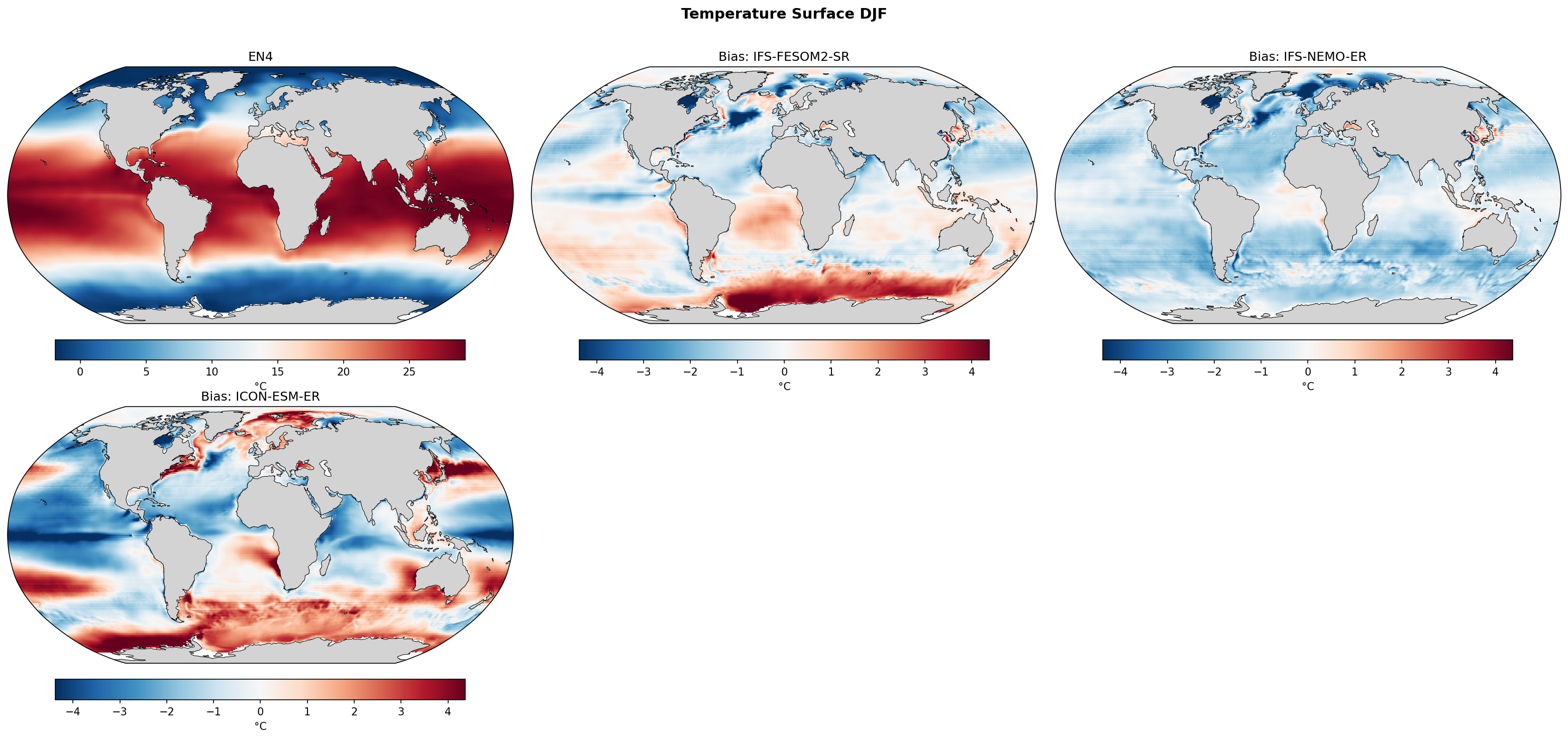
| Variables | thetao, so |
|---|---|
| Models | IFS-FESOM2-SR, IFS-NEMO-ER, ICON-ESM-ER, HadGEM3-GC5 |
| Reference Dataset | EN4 v4.2.2 |
| Units | K |
| Period | 1980–2014 |
| IFS-FESOM2-SR | Global Mean Bias: -0.05 · Rmse: 1.29 |
| IFS-NEMO-ER | Global Mean Bias: -1.04 · Rmse: 1.32 |
| ICON-ESM-ER | Global Mean Bias: -0.30 · Rmse: 2.09 |
| HadGEM3-GC5 | Global Mean Bias: 0.42 · Rmse: 0.99 |
Summary high
This figure evaluates DJF sea surface temperature (SST) biases in three high-resolution coupled models (IFS-FESOM2-SR, IFS-NEMO-ER, ICON-ESM-ER) relative to EN4 observations. While IFS-FESOM2-SR achieves the lowest global mean bias, significant structural differences appear in the North Atlantic and Southern Ocean across the ensemble.
Key Findings
- IFS-NEMO-ER exhibits a pervasive, systematic cold bias across the global ocean (global mean -1.04 K), contrasting with the more regionally compensated biases in the other models.
- ICON-ESM-ER shows the largest regional errors (RMSE ~2.09 K), characterized by a unique, intense warm bias in the subpolar North Atlantic and Labrador Sea, and strong warm biases in the Southern Ocean.
- IFS-FESOM2-SR performs best in terms of global mean bias (-0.05 K) and RMSE (1.29 K) but displays classic warm biases in Eastern Boundary Upwelling Systems (e.g., Benguela, Peru/Chile).
Spatial Patterns
All models show dipolar bias structures in Western Boundary Current regions (Gulf Stream, Kuroshio), indicative of separation latitude errors common even at eddy-permitting resolutions. The Southern Ocean exhibits divergent behavior: a strong warm bias band in ICON-ESM-ER and IFS-FESOM2-SR, versus a cold bias in IFS-NEMO-ER. In the North Atlantic, the 'cold blob' (subpolar cooling) is prominent in both IFS-based models, whereas ICON-ESM-ER shows strong warming there.
Model Agreement
Inter-model agreement is low regarding the sign of biases in key dynamic regions like the Southern Ocean and North Atlantic subpolar gyre. However, there is some agreement on the location of Western Boundary Current separation errors.
Physical Interpretation
The North Atlantic cold bias in IFS models likely reflects a weak Atlantic Meridional Overturning Circulation (AMOC) or excessive surface heat loss, whereas ICON's warm bias there suggests vigorous convective mixing or a displaced North Atlantic Current. The Southern Ocean warm biases in FESOM/ICON are often linked to cloud radiative feedback errors (insufficient reflection of shortwave radiation) or vertical mixing deficiencies. The systematic cold bias in IFS-NEMO-ER suggests a global energy imbalance or initialization drift.
Caveats
- The strong global mean cold bias in IFS-NEMO-ER may mask regional dynamical biases.
- Analysis is restricted to DJF; seasonal compensation in JJA is not visible.
Temperature Surface JJA Bias
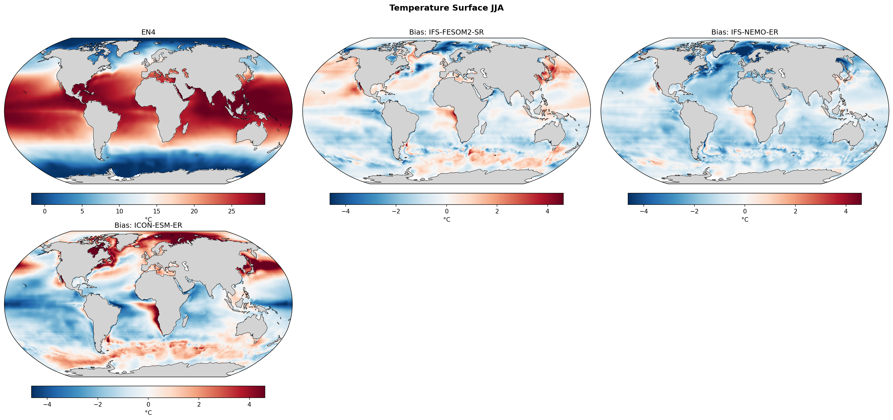
| Variables | thetao, so |
|---|---|
| Models | IFS-FESOM2-SR, IFS-NEMO-ER, ICON-ESM-ER, HadGEM3-GC5 |
| Reference Dataset | EN4 v4.2.2 |
| Units | K |
| Period | 1980–2014 |
| IFS-FESOM2-SR | Global Mean Bias: -0.31 · Rmse: 1.07 |
| IFS-NEMO-ER | Global Mean Bias: -1.06 · Rmse: 1.39 |
| ICON-ESM-ER | Global Mean Bias: -0.41 · Rmse: 1.92 |
| HadGEM3-GC5 | Global Mean Bias: 0.26 · Rmse: 1.00 |
Summary high
This diagnostic compares JJA surface temperature biases of four high-resolution coupled models against EN4 observations. While IFS-NEMO-ER exhibits a severe global cold bias (-1.06°C), HadGEM3-GC5 is the warmest (+0.26°C), and all models struggle with warm biases in eastern boundary upwelling regions.
Key Findings
- IFS-NEMO-ER is dominated by a systematic global cold bias (mean -1.06°C), significantly colder than the other models.
- ICON-ESM-ER displays the highest spatial variability (RMSE 1.92°C), characterised by intense warm biases in the Southern Ocean and Western Boundary Current extensions contrasted with cold tropical biases.
- HadGEM3-GC5 achieves the lowest RMSE (1.00°C) but shows a distinct zonal band of warm bias in the Southern Ocean and widespread warmth in the northern high latitudes.
- Persistent warm biases in eastern boundary upwelling systems (off Peru/Chile and Namibia) are common to all four simulations.
Spatial Patterns
All models show warm biases in the major eastern boundary upwelling zones (Benguela and Humboldt currents). In the North Atlantic, dipole structures suggest difficulties with the Gulf Stream separation and North Atlantic Current path, most notably in ICON and IFS-FESOM. The Southern Ocean reveals a split: ICON and HadGEM3 show strong warm biases (likely sea-ice edge or cloud related), whereas IFS-FESOM and IFS-NEMO are cooler.
Model Agreement
Inter-model agreement is low regarding the global mean state (ranging from -1.1°C to +0.3°C) and Southern Ocean biases. However, there is strong agreement on the location of errors in eastern boundary upwelling regions and Western Boundary Current extensions.
Physical Interpretation
The pervasive warm biases in upwelling regions suggest unresolved coastal dynamics or deficiencies in stratocumulus cloud decks allowing excessive solar heating. The strong warm biases in the Southern Ocean for ICON and HadGEM3 are often linked to cloud phase feedbacks (lack of supercooled liquid water reflecting SW) or shallow mixed layers. The systemic cold bias in IFS-NEMO implies a global energy balance tuning issue, possibly in atmospheric opacity or cloud albedo.
Caveats
- Analysis is restricted to the JJA season (Austral winter), which may amplify Southern Ocean sea-ice edge biases.
- EN4 is an observational analysis product; biases in data-sparse regions like the Southern Ocean should be interpreted with caution.
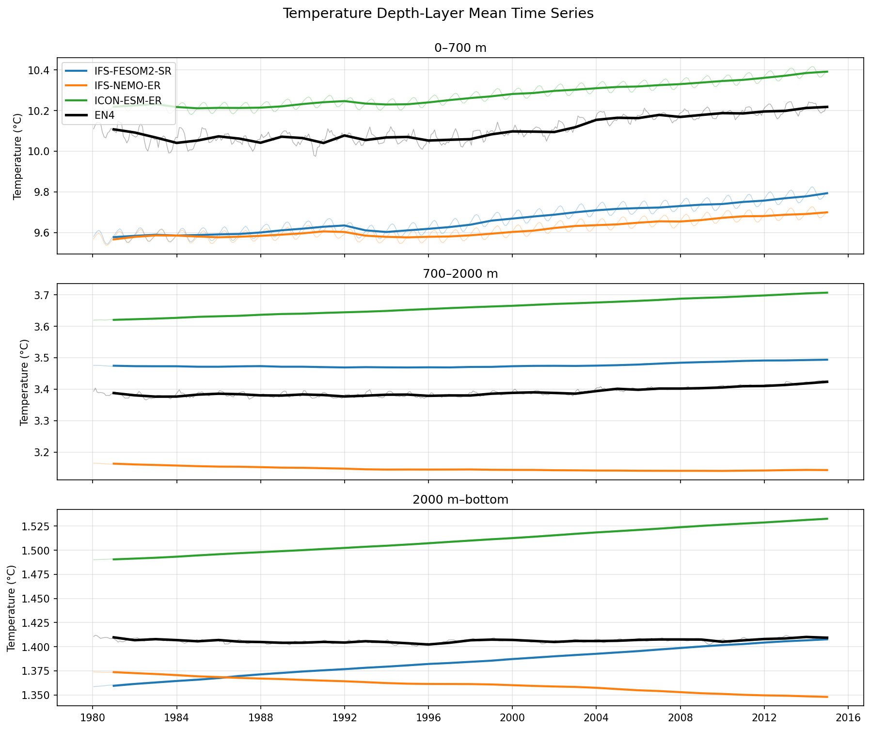
Temperature Depth-Layer Time Series
| Variables | thetao, so |
|---|---|
| Models | IFS-FESOM2-SR, IFS-NEMO-ER, ICON-ESM-ER, HadGEM3-GC5, EN4 |
| Reference Dataset | EN4 v4.2.2 |
| Units | K |
| Period | 1980–2014 |
Summary high
This figure presents time series of global volume-weighted mean ocean temperature for three depth layers (0–700 m, 700–2000 m, >2000 m) over the period 1980–2015, comparing four coupled models against EN4 v4.2.2 observations.
Key Findings
- In the upper ocean (0–700 m), IFS-FESOM2-SR and IFS-NEMO-ER exhibit a persistent cold bias of approximately 0.5°C, while ICON-ESM-ER and HadGEM3-GC5 show a smaller warm bias (~0.1–0.2°C). All models capture the observed warming trend.
- Deep ocean (>2000 m) temperatures reveal significant drifts: ICON-ESM-ER and IFS-FESOM2-SR show strong linear warming trends (drifting away from observations), IFS-NEMO-ER shows a cooling drift, while HadGEM3-GC5 is notably stable and parallel to EN4.
- Mid-ocean (700–2000 m) temperatures show the largest inter-model spread in mean state, with ICON-ESM-ER being the warmest and exhibiting the strongest warming trend, contrasting with the cooling trend in IFS-NEMO-ER.
Spatial Patterns
The warming signal is primarily confined to the upper ocean (0–700 m) in observations and HadGEM3-GC5. However, ICON-ESM-ER and IFS-FESOM2-SR allow this warming signal (or spurious drift) to penetrate effectively into the deep ocean layers.
Model Agreement
Models generally agree on the sign of the upper-ocean warming trend but disagree significantly on the mean state (offsets of up to ~0.7°C between ICON and IFS). Agreement degrades with depth, with models diverging in both mean state and trend direction in the deep ocean.
Physical Interpretation
The clustering of the two IFS-based models (IFS-FESOM2-SR and IFS-NEMO-ER) in the upper ocean (both cold biased) despite different ocean components suggests the bias is driven by the IFS atmospheric component or surface flux coupling. Conversely, the divergence in the deep ocean between these two (FESOM warming vs NEMO cooling) points to ocean-model-specific drift or initialization issues (spin-up). ICON-ESM-ER appears to have a net positive energy imbalance driving warming throughout the column.
Caveats
- Deep ocean observational data (EN4) becomes sparser back in time, increasing uncertainty in the reference trend.
- Linear drifts in the deep ocean suggest some models (ICON, IFS-FESOM) have not reached quasi-equilibrium, which may contaminate estimates of anthropogenic heat uptake.
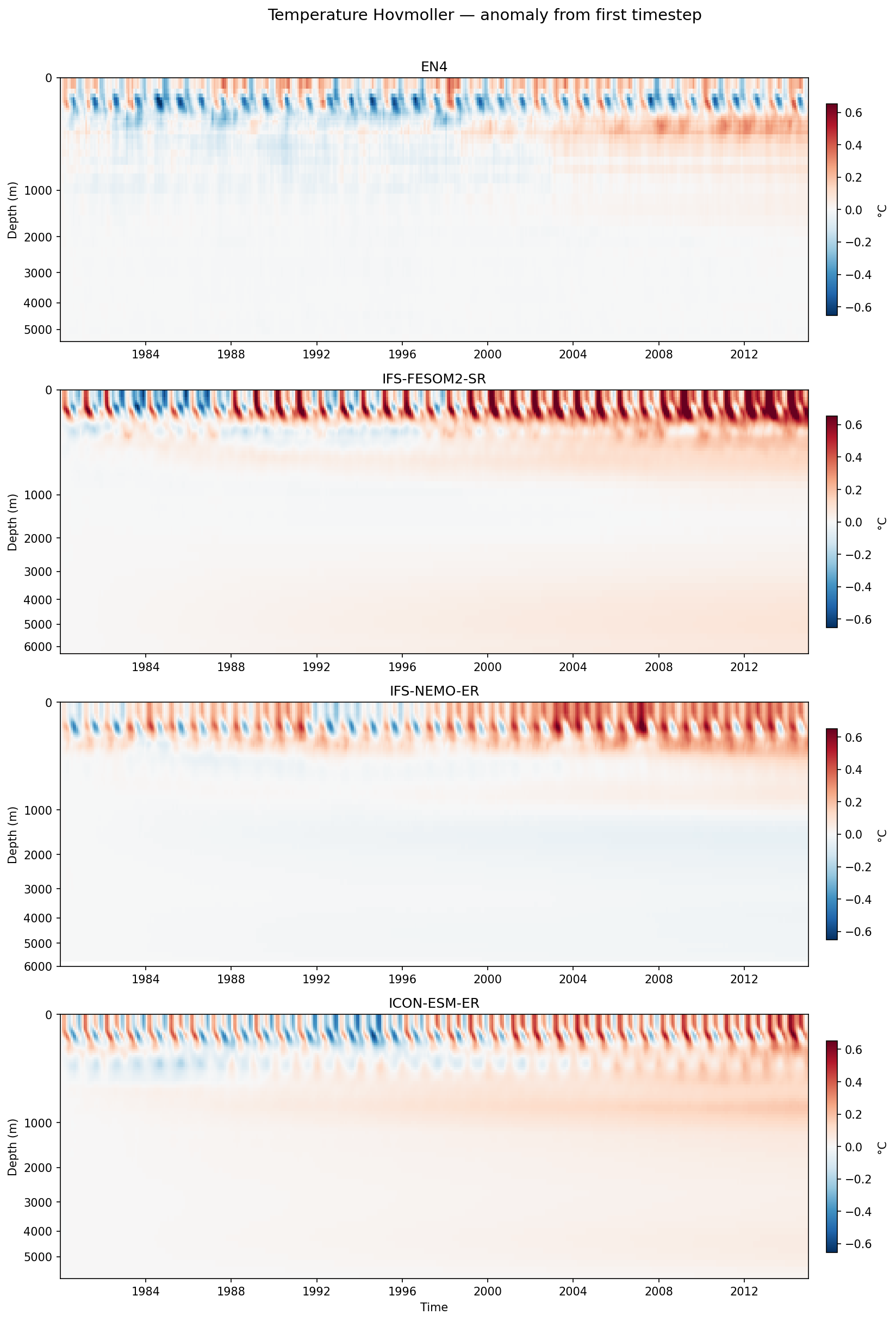
Temperature Hovmoller (first-timestep anomaly)
| Variables | thetao, so |
|---|---|
| Models | IFS-FESOM2-SR, IFS-NEMO-ER, ICON-ESM-ER, HadGEM3-GC5 |
| Reference Dataset | EN4 v4.2.2 |
| Units | K |
| Period | 1980–2014 |
Summary high
This time-depth Hovmoller diagram compares the evolution of global mean ocean temperature anomalies (relative to the initial 1980 timestep) in EN4 observations against four high-resolution coupled models. While all datasets show upper-ocean warming consistent with anthropogenic forcing, the models exhibit significant differences in vertical heat penetration and initialization drift.
Key Findings
- HadGEM3-GC5 exhibits the most aggressive warming, with anomalies exceeding 0.6 K penetrating rapidly below 1000 m, significantly overestimating the heat uptake compared to EN4.
- IFS-NEMO-ER displays a unique and substantial cooling drift in the intermediate ocean (approx. 1000–3000 m), contrasting with the warming or neutral signals in all other models and observations.
- EN4 observations show warming primarily concentrated in the upper 700 m, whereas IFS-FESOM2-SR and ICON-ESM-ER show warming signals penetrating deeper (to ~1500 m and ~1000 m respectively).
- ICON-ESM-ER maintains the most stable deep ocean (>2000 m) compared to the diffusive warming drift seen in IFS-FESOM2-SR and HadGEM3-GC5.
Spatial Patterns
The dominant pattern is a surface-intensified warming trend propagating downwards over time. Strong annual periodicity (vertical striping) is visible in the upper 200 m for all models, representing the seasonal cycle. The warming signal in EN4 is notably more stratified/confined to the upper layers compared to the more diffusive vertical propagation in the models.
Model Agreement
All models agree on the sign of the surface trend (warming), but diverge strongly in the intermediate and deep ocean. Inter-model spread is largest between the cooling intermediate layer of IFS-NEMO-ER and the intense deep warming of HadGEM3-GC5.
Physical Interpretation
The plots conflate forced climate change (surface heating) with model drift. The deep warming in HadGEM3-GC5 and IFS-FESOM2-SR suggests rapid vertical mixing or initialization shock where the model climatology is warmer than the initial state. The intermediate cooling in IFS-NEMO-ER likely reflects an adjustment in the Atlantic Meridional Overturning Circulation (AMOC) or water mass ventilation properties (e.g., changes in North Atlantic Deep Water formation) specific to the NEMO configuration.
Caveats
- The metric 'anomaly from first timestep' makes it difficult to separate anthropogenic warming trends from intrinsic model drift.
- Since these are free-running coupled simulations, the phase of internal variability (e.g., ENSO events visible as vertical streaks in EN4) is not expected to match observations.
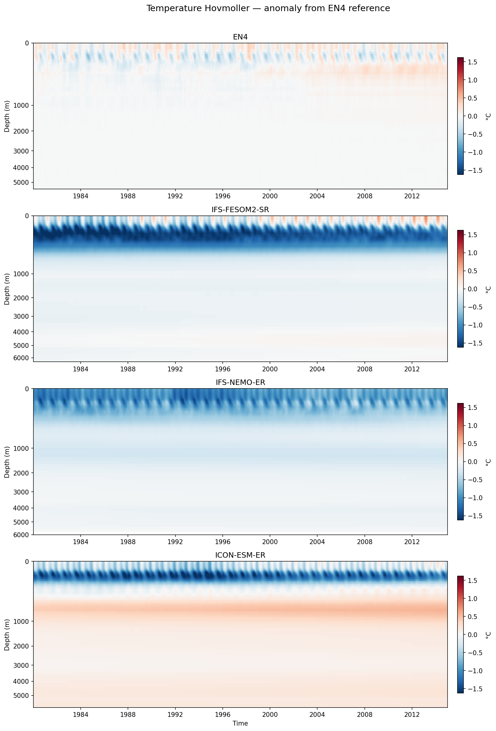
Temperature Hovmoller (EN4-ref anomaly)
| Variables | thetao, so |
|---|---|
| Models | IFS-FESOM2-SR, IFS-NEMO-ER, ICON-ESM-ER, HadGEM3-GC5 |
| Reference Dataset | EN4 v4.2.2 |
| Units | K |
| Period | 1980–2014 |
Summary high
Time-depth Hovmoller diagrams illustrate the evolution of global ocean temperature anomalies relative to the EN4 1980 reference profile, revealing that model drifts significantly outweigh the observed warming signal over the 1980–2014 period.
Key Findings
- IFS-FESOM2-SR and IFS-NEMO-ER exhibit a strong, rapid cooling drift (cold bias) in the upper 800 m, with anomalies reaching -1.0°C to -1.5°C, effectively masking any historical warming trend.
- ICON-ESM-ER develops a distinct vertical dipole bias: cooling in the top 400 m contrasted by a prominent band of warming (+0.5°C to +1.0°C) at intermediate depths (500–1500 m).
- HadGEM3-GC5 contrasts with other models by showing excessive warming in the upper 500 m relative to EN4, coupled with a mild cooling drift at intermediate depths (1000–3000 m).
- Observational data (EN4) shows a modest, gradual warming signal penetrating from the surface, which is qualitatively different from the structural drifts seen in the simulations.
Spatial Patterns
Biases are strongly stratified by depth. The IFS models show surface-intensified cooling extending into the thermocline. ICON's anomaly is structurally unique with its 'sandwich' of cold surface, warm intermediate, and deep warming. HadGEM3 shows surface-intensified warming.
Model Agreement
Low agreement on the sign and vertical structure of ocean drift. While IFS variants behave similarly (cold upper ocean), ICON (subsurface warming) and HadGEM3 (surface warming) show fundamentally different drift regimes.
Physical Interpretation
The rapid onset of these anomalies suggests initialization shock or systematic imbalances in surface energy fluxes and vertical mixing. The cold drift in IFS models implies insufficient heat retention or excessive surface loss. ICON's intermediate warming band may result from issues in parameterizing vertical mixing or ventilation of intermediate waters (e.g., overflow parameterizations). HadGEM3's warm surface drift suggests a positive net surface energy imbalance or reduced efficiency in transporting heat to the deep ocean.
Caveats
- The anomalies are relative to the initial observational state (EN4), conflating model drift with the transient climate change signal; however, the magnitude of model drift appears to dominate.
- The depth axis is likely non-linear (emphasizing the upper ocean), which visually compresses deep ocean drifts.