Evaluation Seasonal Cycle CMIP6
CMIP6 Multi-Model Mean Context
Comparison with CMIP6 ensemble mean from 11 members.
Contributing models: ACCESS-ESM1-5, AWI-CM-1-1-MR, CNRM-CM6-1, CNRM-ESM2-1, EC-Earth3, FGOALS-g3, GISS-E2-1-G, INM-CM5-0, IPSL-CM6A-LR, MPI-ESM1-2-LR, MRI-ESM2-0
Synthesis
Related diagnostics
Total Cloud Cover Seasonal Cycle
| Variables | clt |
|---|---|
| Models | IFS-FESOM2-SR, IFS-NEMO-ER, ICON-ESM-ER, HadGEM3-GC5, MPI-ESM1-2-LR, GISS-E2-1-G, IPSL-CM6A-LR, ACCESS-ESM1-5, EC-Earth3, CNRM-CM6-1, AWI-CM-1-1-MR, CNRM-ESM2-1, FGOALS-g3, INM-CM5-0, MRI-ESM2-0 |
| Reference Dataset | ERA5 |
| Units | % |
| Period | 1980–2014 |
Summary high
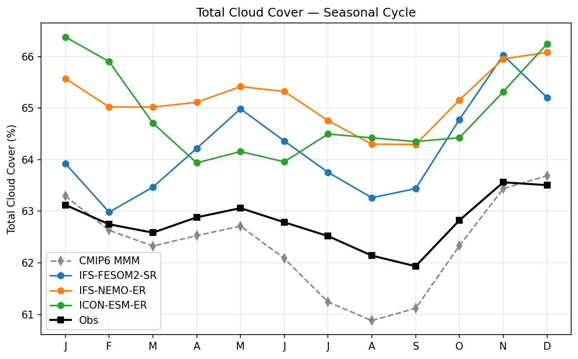
This figure compares the seasonal cycle of global-mean Total Cloud Cover (TCC) in four high-resolution coupled models against ERA5 reanalysis and the CMIP6 ensemble.
Key Findings
- All four evaluated high-resolution models exhibit a positive bias in global-mean cloud cover relative to ERA5.
- HadGEM3-GC5 is a significant outlier with a severe positive bias of approximately 8-10%, showing values around 72% compared to the ERA5 baseline of ~63%.
- IFS-FESOM2-SR demonstrates the highest skill, tracking the ERA5 magnitude and phase most closely (bias < 1%), while IFS-NEMO-ER and ICON-ESM-ER show moderate positive biases of 2-3%.
Spatial Patterns
The global seasonal cycle exhibits a characteristic minimum in boreal late summer (August-September) and a maximum in boreal winter (December-January). This phase is generally captured by all models, though amplitudes vary.
Model Agreement
There is significant inter-model spread. IFS-FESOM2-SR agrees best with observations. The CMIP6 Multi-Model Mean tends to slightly underestimate TCC (negative bias), contrasting with the high-resolution models which all overestimate it. The spread within the CMIP6 ensemble is very large (~20%).
Physical Interpretation
The positive biases, particularly in HadGEM3, suggest overly aggressive cloud formation parameterizations (likely low-level stratocumulus or convective detrainment). The difference between IFS-FESOM2 and IFS-NEMO (which share atmospheric physics) implies that air-sea coupling differences (SST biases) or tuning choices specific to the ocean component significantly modulate global cloudiness.
Caveats
- Global mean values can mask compensating regional biases (e.g., excess polar clouds vs. deficit in stratocumulus decks).
- ERA5 cloud cover is a forecast product, not directly assimilated, though it is considered a high-quality reference.
Surface Latent Heat Flux Seasonal Cycle
| Variables | hfls |
|---|---|
| Models | IFS-FESOM2-SR, IFS-NEMO-ER, ICON-ESM-ER, HadGEM3-GC5 |
| Reference Dataset | ERA5 |
| Units | W/m2 |
| Period | 1980–2014 |
Summary high
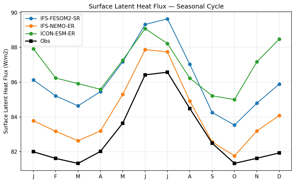
This figure shows the seasonal cycle of global mean surface latent heat flux, revealing that all three high-resolution models systematically overestimate the flux compared to ERA5 reanalysis. While the phase of the seasonal cycle—peaking in June-July—is generally captured, the magnitude of the model biases varies, with ICON-ESM-ER showing the largest discrepancies, particularly in boreal winter.
Key Findings
- All models exhibit a positive bias (excessive evaporation) relative to ERA5 throughout the entire year.
- IFS-NEMO-ER is the best-performing model, tracking ERA5 most closely with a bias of ~+1–2 W/m², particularly converging with observations in September–October.
- ICON-ESM-ER shows the largest bias (~+6 W/m²) during December–January, failing to reproduce the observed seasonal minimum in these months.
- The seasonal maximum occurs in June–July for all datasets, consistent with strong fluxes in the Southern Hemisphere winter.
Spatial Patterns
The global mean cycle is bimodal in ERA5 with minima in March and October and a broad maximum in June–July. Models generally reproduce this shape, although ICON-ESM-ER deviates significantly in shape during November–January by maintaining high flux values instead of dropping.
Model Agreement
Models agree on the timing of the mid-year maximum (June-July) but disagree on the magnitude of the flux and the shape of the cycle in boreal winter. IFS-FESOM2-SR and IFS-NEMO-ER share a very similar seasonal shape (shifted by constant offset), whereas ICON-ESM-ER diverges in behavior during DJF.
Physical Interpretation
The systematic positive bias suggests these high-resolution models maintain excessive evaporation, likely driven by warm Sea Surface Temperature (SST) biases often found in these simulations (e.g., in the Southern Ocean or upwelling zones) or stronger-than-observed surface winds. The distinct DJF bias in ICON-ESM-ER suggests specific issues with wintertime evaporation, possibly in Northern Hemisphere western boundary currents (Gulf Stream/Kuroshio) where latent heat loss is maximized in winter.
Caveats
- ERA5 is a reanalysis product and has its own uncertainties regarding surface fluxes.
- HadGEM3-GC5 is listed in the metadata but does not appear in the legend or plot.
- Global means mask potential regional error cancellations (e.g., tropical vs. high-latitude biases).
Surface Sensible Heat Flux Seasonal Cycle
| Variables | hfss |
|---|---|
| Models | IFS-FESOM2-SR, IFS-NEMO-ER, ICON-ESM-ER, HadGEM3-GC5 |
| Reference Dataset | ERA5 |
| Units | W/m2 |
| Period | 1980–2014 |
Summary high
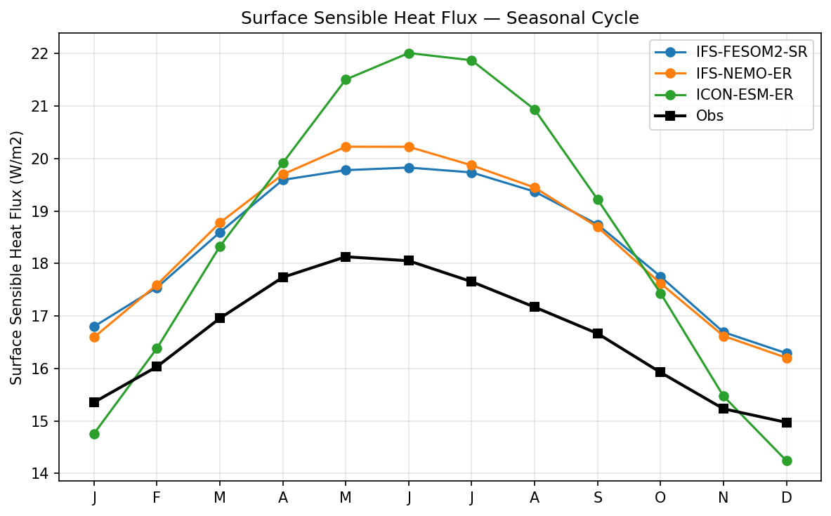
The figure illustrates the global mean seasonal cycle of surface sensible heat flux (SSH), showing that while models capture the general phase peaking in boreal summer, they exhibit distinct amplitude and magnitude biases relative to ERA5.
Key Findings
- IFS-FESOM2-SR and IFS-NEMO-ER consistently overestimate global mean SSH by approximately 1.5–2.5 W/m² throughout the year relative to ERA5.
- ICON-ESM-ER exhibits an exaggerated seasonal cycle amplitude, matching ERA5 closely in boreal winter (~14–15 W/m²) but significantly overshooting the summer peak by ~4 W/m² (reaching 22 W/m² vs ERA5's 18 W/m²).
- The two IFS-based models show nearly identical behavior, indicating that the atmospheric model formulation (IFS) dominates the sensible heat flux characteristics rather than the specific ocean coupling (FESOM vs. NEMO).
Spatial Patterns
The seasonal cycle follows the Northern Hemisphere solar cycle (peaking June-July), reflecting the dominance of NH land masses on the global mean sensible heat flux. ICON displays the sharpest temporal gradients (strongest warming trend in spring).
Model Agreement
Models generally agree on the phase (timing of max/min) but disagree on magnitude. IFS models are systematically high year-round; ICON is high in summer but accurate in winter.
Physical Interpretation
The systematic positive bias suggests models maintain a larger surface-to-air temperature gradient or employ higher turbulent transfer coefficients than the reanalysis. ICON's excessive summer peak likely indicates a Bowen ratio bias over Northern Hemisphere land (favoring sensible over latent heat), potentially due to soil moisture drying or land-surface coupling strength.
Caveats
- HadGEM3-GC5 is listed in the metadata but is missing from the figure legend and plot.
- Global averaging masks potential regional compensations between ocean and land fluxes.
Total Precipitation Rate Seasonal Cycle
| Variables | pr |
|---|---|
| Models | IFS-FESOM2-SR, IFS-NEMO-ER, ICON-ESM-ER, HadGEM3-GC5, MPI-ESM1-2-LR, GISS-E2-1-G, IPSL-CM6A-LR, ACCESS-ESM1-5, EC-Earth3, CNRM-CM6-1, AWI-CM-1-1-MR, CNRM-ESM2-1, FGOALS-g3, INM-CM5-0, MRI-ESM2-0 |
| Reference Dataset | ERA5 |
| Units | kg/m2/s |
| Period | 1980–2014 |
Summary high
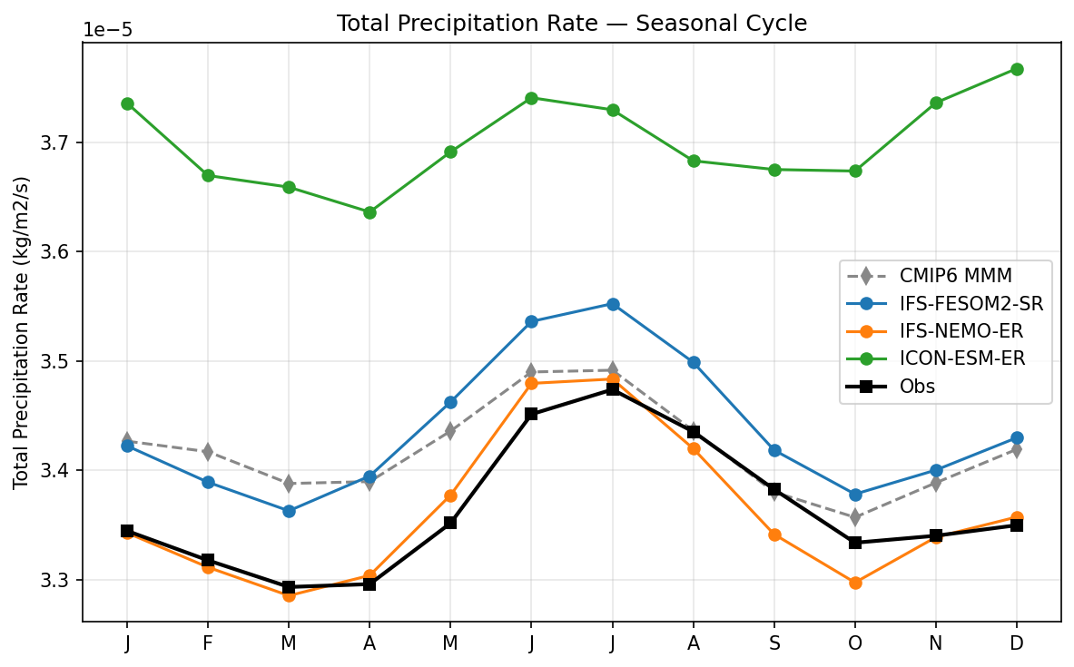
The figure illustrates the seasonal cycle of global mean total precipitation rate for four EERIE models compared to ERA5 reanalysis and the CMIP6 ensemble. There is a significant divergence in mean precipitation rates among the models, despite general agreement on the seasonal phase.
Key Findings
- IFS-NEMO-ER shows excellent agreement with ERA5, closely matching both the climatological mean magnitude and the seasonal amplitude/phase.
- ICON-ESM-ER and HadGEM3-GC5 exhibit a substantial systematic wet bias, with global mean precipitation rates approximately 10% higher than ERA5 (around 3.7e-5 vs 3.4e-5 kg/m²/s).
- IFS-FESOM2-SR overestimates precipitation relative to ERA5 but lies closer to observations than ICON or HadGEM3, falling near the upper range of the CMIP6 multi-model mean.
- All models capture the correct seasonal phasing with a global minimum in March and a maximum in July, though amplitudes vary.
Spatial Patterns
The global mean seasonal cycle is characterized by a peak in boreal summer (July) and a minimum in boreal spring (March), reflecting the dominance of Northern Hemisphere land-driven precipitation patterns (e.g., monsoons) on the global average.
Model Agreement
Inter-model spread is large regarding the mean state. IFS-NEMO-ER provides the best match to observations. HadGEM3-GC5 and ICON-ESM-ER are significant outliers on the high (wet) side, exceeding the values of most CMIP6 ensemble members.
Physical Interpretation
The large wet bias in ICON-ESM-ER and HadGEM3-GC5 suggests an overly active hydrologic cycle, which implies that global evaporation and precipitation are spinning too fast. This is fundamentally constrained by the atmospheric radiative cooling rate; thus, these models may have compensating errors in surface energy fluxes or radiative cooling.
Caveats
- Global mean precipitation in reanalyses (ERA5) relies heavily on the model physics and data assimilation, as direct global observation (especially over oceans) is difficult; however, the bias in ICON/HadGEM3 is large enough to be considered robust.
Mean Sea Level Pressure Seasonal Cycle
| Variables | psl |
|---|---|
| Models | IFS-FESOM2-SR, IFS-NEMO-ER, ICON-ESM-ER, HadGEM3-GC5, MPI-ESM1-2-LR, GISS-E2-1-G, IPSL-CM6A-LR, ACCESS-ESM1-5, EC-Earth3, CNRM-CM6-1, AWI-CM-1-1-MR, CNRM-ESM2-1, FGOALS-g3, INM-CM5-0, MRI-ESM2-0 |
| Reference Dataset | ERA5 |
| Units | Pa |
| Period | 1980–2014 |
Summary high
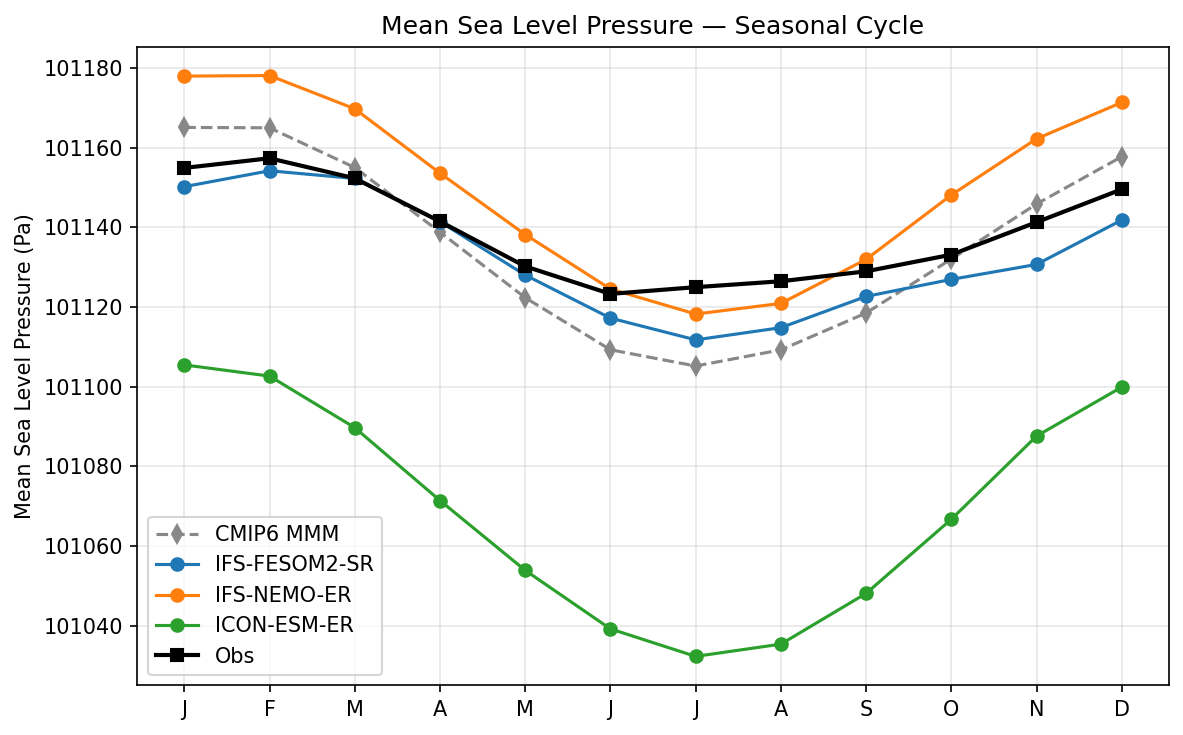
The figure illustrates the seasonal cycle of global mean Mean Sea Level Pressure (MSLP), revealing significant systematic offsets in total atmospheric mass or pressure reduction between the models despite good agreement on the seasonal phase.
Key Findings
- ICON-ESM-ER exhibits a large, systematic negative bias of approximately 80-100 Pa (~1 hPa) relative to ERA5 throughout the annual cycle.
- IFS-NEMO-ER shows a consistent positive bias of roughly 20-30 Pa, while IFS-FESOM2-SR tracks closest to observations, showing a small negative bias (<10 Pa).
- All models and the CMIP6 MMM correctly capture the phase of the seasonal cycle, with a global minimum in boreal summer (June-July) and maximum in boreal winter (December-January).
- The CMIP6 Multi-Model Mean exaggerates the amplitude of the seasonal cycle, with a deeper minimum in summer compared to ERA5 and the high-resolution IFS models.
Spatial Patterns
While this is a global-mean time series, the temporal pattern shows a distinct seasonal cycle driven by Northern Hemisphere land-sea thermal contrasts. The global mean MSLP is lowest in JJA, consistent with the 'thermal low' effect where reduction to sea level under warm conditions over large NH landmasses results in lower calculated pressures.
Model Agreement
There is strong agreement on the phase of the seasonal cycle across all datasets. However, there is significant disagreement on the absolute magnitude (the global mean state), with a spread of nearly 1.5 hPa between the highest (IFS-NEMO-ER) and lowest (ICON-ESM-ER) models. IFS-FESOM2-SR provides the best match to the ERA5 amplitude and mean state.
Physical Interpretation
The seasonal variation is primarily an artifact of the mathematical reduction of surface pressure to sea level; warmer temperatures in the NH summer (dominated by land) lead to lower reduced pressures (thermal lows). The constant offsets between models likely stem from differences in the total atmospheric mass initialization or conservation (tuning of the dry air mass) rather than dynamical feedback errors. The slight difference between IFS-NEMO and IFS-FESOM (which share the same atmosphere) implies influence from the underlying ocean/ice state or coupling frequency on the global pressure integration or water vapor loading.
Caveats
- Global mean MSLP is a calculated quantity dependent on reduction algorithms over topography, not a direct measurement of total atmospheric mass (which is Surface Pressure).
- The large bias in ICON may be a static initialization offset rather than a process drift.
Surface Downwelling Longwave Seasonal Cycle
| Variables | rlds |
|---|---|
| Models | IFS-FESOM2-SR, IFS-NEMO-ER, ICON-ESM-ER, HadGEM3-GC5, MPI-ESM1-2-LR, GISS-E2-1-G, IPSL-CM6A-LR, ACCESS-ESM1-5, EC-Earth3, CNRM-CM6-1, AWI-CM-1-1-MR, CNRM-ESM2-1, FGOALS-g3, INM-CM5-0, MRI-ESM2-0 |
| Reference Dataset | ERA5 |
| Units | W/m2 |
| Period | 1980–2014 |
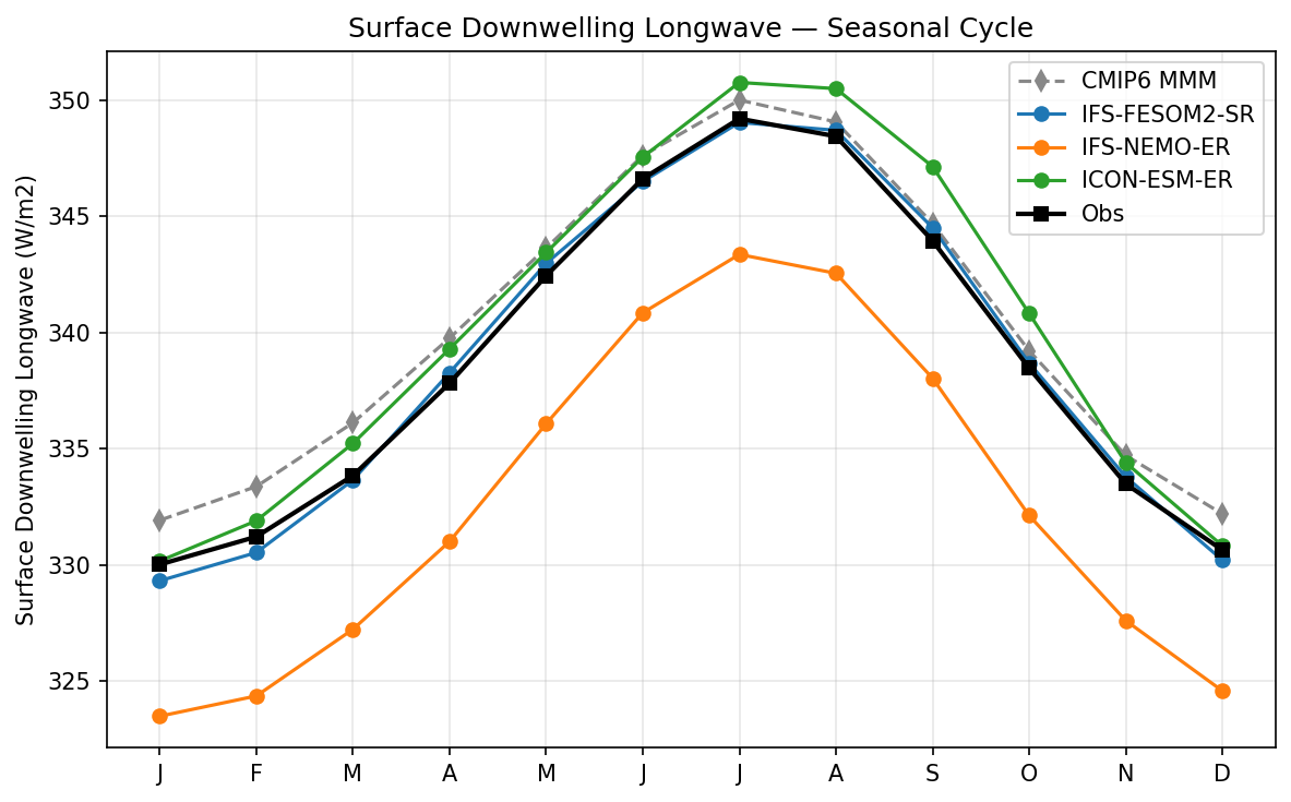
Summary high
The figure illustrates the seasonal cycle of global mean surface downwelling longwave radiation (rlds), comparing three high-resolution models against ERA5 and the CMIP6 ensemble. IFS-FESOM2-SR demonstrates exceptional skill, while IFS-NEMO-ER and ICON-ESM-ER show distinct negative and positive biases, respectively.
Key Findings
- IFS-FESOM2-SR shows remarkable agreement with ERA5, tracking the observational reference almost perfectly throughout the year with negligible bias (< 1 W/m²).
- IFS-NEMO-ER exhibits a systematic negative bias of approximately 6–7 W/m² across all months, falling near the lower bound of the CMIP6 ensemble spread.
- ICON-ESM-ER tends to overestimate downwelling longwave, particularly during the boreal summer peak (~351 W/m² vs ~349 W/m² in ERA5), aligning closely with the CMIP6 Multi-Model Mean.
- All models correctly capture the phase of the seasonal cycle, with the global minimum in January and maximum in July.
Spatial Patterns
The seasonal cycle follows the Northern Hemisphere temperature cycle (peaking in July), reflecting the dominance of NH landmasses on global mean temperature and atmospheric humidity. The amplitude of the cycle is roughly 20 W/m² (from ~330 to ~350 W/m²).
Model Agreement
While phase agreement is high, amplitude and mean state vary significantly. IFS-FESOM2-SR outperforms the CMIP6 Multi-Model Mean. In contrast, IFS-NEMO-ER is a notable outlier on the low side compared to the other high-res models, though it remains within the full CMIP6 range.
Physical Interpretation
Surface downwelling longwave radiation is primarily a function of lower-tropospheric temperature, water vapor content, and cloud cover. IFS-NEMO-ER's substantial negative bias suggests a globally cooler atmosphere, a dry bias (insufficient water vapor), or underestimated cloud fraction relative to ERA5. Conversely, ICON-ESM-ER's positive bias implies a warmer, moister atmosphere or excessive cloudiness. The divergence between IFS-NEMO-ER and IFS-FESOM2-SR is notable given they likely share similar atmospheric physics, pointing to coupled ocean-atmosphere feedback differences (e.g., cooler SSTs in IFS-NEMO-ER leading to reduced evaporation and greenhouse forcing).
Caveats
- The observational reference is ERA5 reanalysis; while robust, comparisons against CERES EBAF could provide additional validation.
- Global mean values can mask compensating regional biases (e.g., cancelling errors between tropics and poles).
Surface Downwelling Shortwave Seasonal Cycle
| Variables | rsds |
|---|---|
| Models | IFS-FESOM2-SR, IFS-NEMO-ER, ICON-ESM-ER, HadGEM3-GC5, MPI-ESM1-2-LR, GISS-E2-1-G, IPSL-CM6A-LR, ACCESS-ESM1-5, EC-Earth3, CNRM-CM6-1, AWI-CM-1-1-MR, CNRM-ESM2-1, FGOALS-g3, INM-CM5-0, MRI-ESM2-0 |
| Reference Dataset | ERA5 |
| Units | W/m2 |
| Period | 1980–2014 |
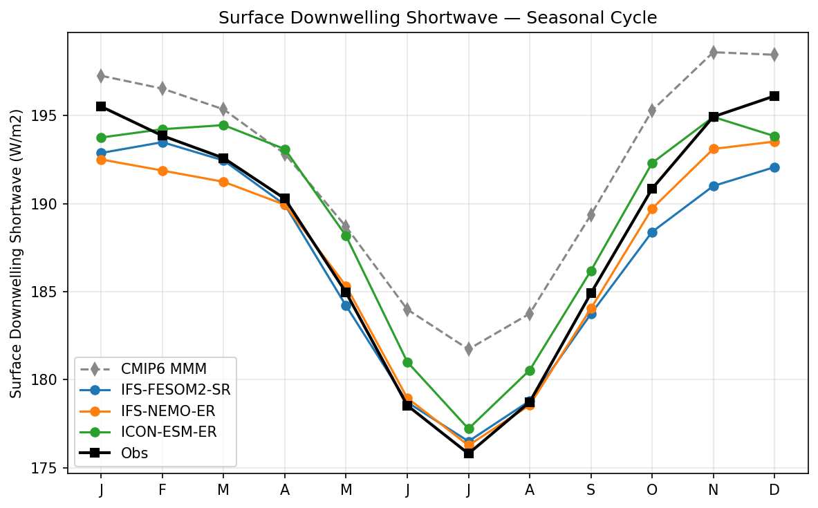
Summary high
This figure displays the seasonal cycle of global mean surface downwelling shortwave radiation (rsds), revealing that the high-resolution EERIE models (especially IFS variants) align much more closely with ERA5 observations than the CMIP6 Multi-Model Mean.
Key Findings
- The CMIP6 Multi-Model Mean (MMM) exhibits a systematic positive bias of approximately 3–6 W/m² throughout the year compared to ERA5 observations.
- IFS-NEMO-ER demonstrates the strongest agreement with observations, closely tracking the ERA5 seasonal cycle with deviations generally under 1 W/m².
- ICON-ESM-ER shows a positive bias relative to observations during transition months (March-May and October-November) but aligns well during the solstice months.
- The seasonal amplitude (January maximum vs. July minimum) is accurately captured by the EERIE models (~19 W/m² range), whereas the CMIP6 MMM shows a damped amplitude (~16 W/m²).
Spatial Patterns
The temporal pattern follows the Earth's orbital eccentricity, with maximum global insolation near perihelion (January) and minimum near aphelion (July).
Model Agreement
High-resolution models cluster closer to observations than the coarse-resolution CMIP6 ensemble. Within the EERIE group, IFS-NEMO-ER and IFS-FESOM2-SR show high consistency in summer but diverge slightly in winter, while ICON-ESM-ER is an outlier with higher values in spring/autumn.
Physical Interpretation
The pervasive positive bias in CMIP6 suggests an underestimation of atmospheric attenuation (likely due to insufficient cloud cover or optical thickness), leading to excessive solar radiation reaching the surface. The EERIE models appear to correct this 'surface brightening' bias, potentially due to improved cloud parameterizations or resolution-dependent dynamics. The seasonal cycle itself is driven by the variation in solar distance.
Caveats
- Global averaging masks potential regional compensating errors (e.g., biases in specific cloud regimes).
- The observational reference is ERA5 reanalysis; comparisons with direct satellite products (like CERES) would validate the reanalysis accuracy.
2m Temperature Seasonal Cycle
| Variables | tas |
|---|---|
| Models | IFS-FESOM2-SR, IFS-NEMO-ER, ICON-ESM-ER, HadGEM3-GC5, MPI-ESM1-2-LR, GISS-E2-1-G, IPSL-CM6A-LR, ACCESS-ESM1-5, EC-Earth3, CNRM-CM6-1, AWI-CM-1-1-MR, CNRM-ESM2-1, FGOALS-g3, INM-CM5-0, MRI-ESM2-0 |
| Reference Dataset | ERA5 |
| Units | K |
| Period | 1980–2014 |
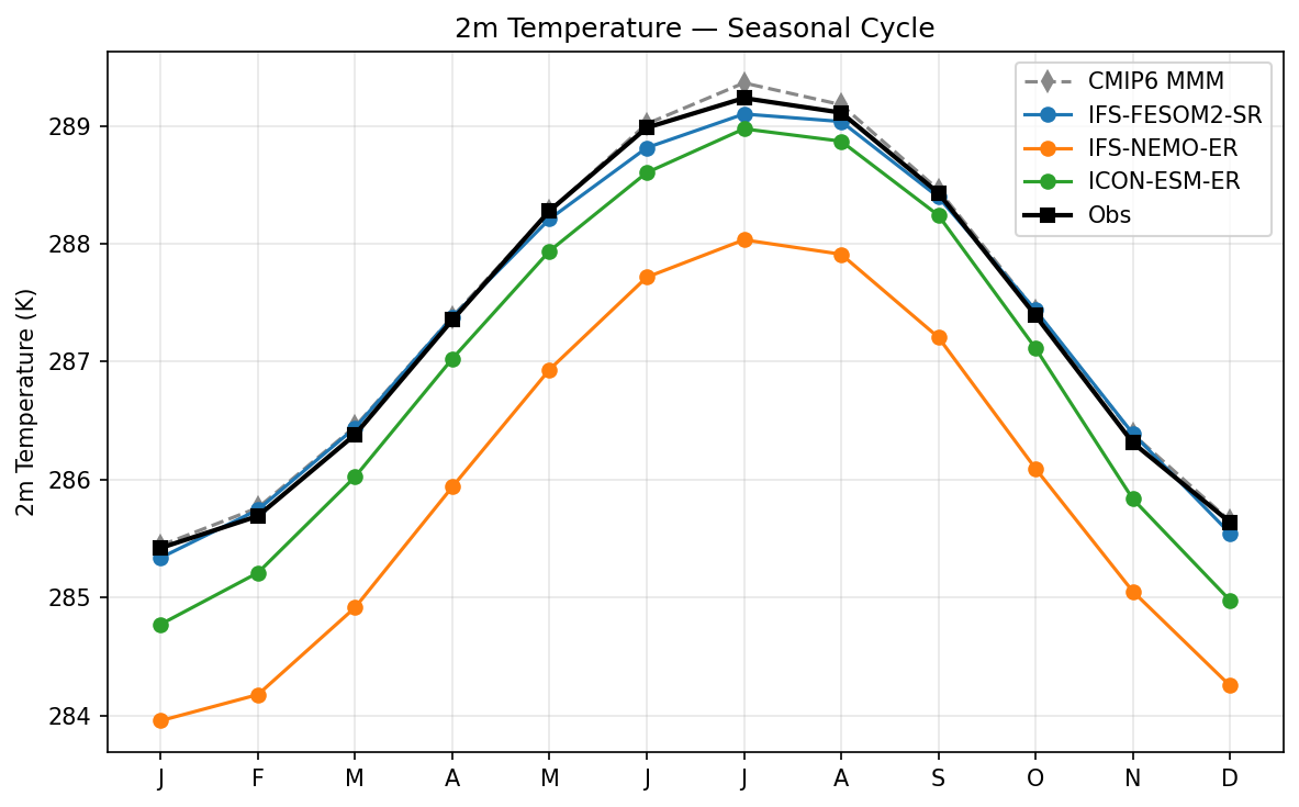
Summary high
This figure displays the climatological annual cycle of global mean 2-meter temperature, revealing distinct systematic biases across the high-resolution models relative to ERA5.
Key Findings
- IFS-FESOM2-SR exhibits excellent skill, tracking the ERA5 reference almost perfectly (within ~0.1 K) throughout the seasonal cycle.
- IFS-NEMO-ER shows a severe systematic cold bias of approximately 1.2 to 1.4 K year-round, falling notably below the entire envelope of CMIP6 ensemble members.
- HadGEM3-GC5 displays a consistent warm bias of roughly 0.6–0.9 K, positioning it at or above the upper bound of the CMIP6 ensemble spread.
- ICON-ESM-ER shows a moderate cold bias (~0.6 K in Jan, ~0.2 K in July), with a slightly dampened seasonal amplitude compared to observations.
Spatial Patterns
All models capture the correct phase of the seasonal cycle, with a minimum in January (~285.4 K in ERA5) and a maximum in July (~289.2 K in ERA5), driven by the Northern Hemisphere's larger land fraction dominating the global mean signal.
Model Agreement
Inter-model spread is significant (~2 K between the warmest and coldest models), exceeding the CMIP6 multi-model mean spread. IFS-FESOM2-SR aligns best with ERA5 and the CMIP6 MMM, while IFS-NEMO-ER is a distinct cold outlier.
Physical Interpretation
The seasonal cycle amplitude is controlled by the thermal inertia difference between land and ocean. The persistent offsets (biases) suggest systematic errors in the planetary energy budget rather than seasonal forcing errors. The severe cold bias in IFS-NEMO-ER could stem from initialization shock, strong ocean heat uptake, or tuning of cloud radiative parameters, whereas HadGEM3-GC5's warm bias may relate to high equilibrium climate sensitivity or insufficient low-cloud cooling.
Caveats
- Global mean values can mask significant compensating regional biases (e.g., a warm Arctic cancelling a cold Tropics).
- The cause of IFS-NEMO-ER's cold bias requires investigation into ocean spin-up or radiative tuning specific to that configuration.
10m U Wind Seasonal Cycle
| Variables | uas |
|---|---|
| Models | IFS-FESOM2-SR, IFS-NEMO-ER, ICON-ESM-ER, HadGEM3-GC5, MPI-ESM1-2-LR, GISS-E2-1-G, IPSL-CM6A-LR, ACCESS-ESM1-5, EC-Earth3, CNRM-CM6-1, AWI-CM-1-1-MR, CNRM-ESM2-1, INM-CM5-0, MRI-ESM2-0 |
| Reference Dataset | ERA5 |
| Units | m/s |
| Period | 1980–2014 |
Summary high
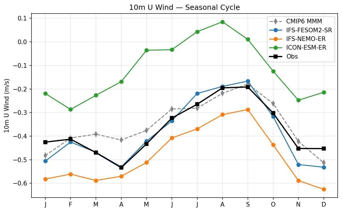
This figure evaluates the seasonal cycle of global-mean 10m zonal (U) wind in four high-resolution EERIE models compared to ERA5 reanalysis and the CMIP6 ensemble.
Key Findings
- IFS-FESOM2-SR shows remarkable agreement with ERA5, capturing both the phase and amplitude of the seasonal cycle almost perfectly, with only a negligible negative bias in boreal winter.
- ICON-ESM-ER exhibits a distinct positive systematic bias (~0.2-0.3 m/s), making the global mean wind significantly more westerly (or less easterly) than observed, even becoming positive in boreal summer.
- IFS-NEMO-ER displays a systematic negative bias (~0.15 m/s) relative to ERA5, consistently showing stronger net easterlies throughout the year.
- HadGEM3-GC5 tracks the CMIP6 multi-model mean closely, showing a slight positive bias relative to ERA5 but capturing the seasonal phase well.
Spatial Patterns
The global mean 10m U wind is negative (easterly dominated) throughout the year in observations, reaching a minimum (strongest easterlies) in April (~-0.55 m/s) and a maximum (weakest easterlies) in September (~-0.2 m/s). This seasonality is likely driven by the strengthening of Southern Hemisphere westerlies in austral winter/spring.
Model Agreement
Inter-model spread is large relative to the mean signal (~0.6 m/s spread vs ~0.4 m/s amplitude). IFS-FESOM2-SR is the best performer. Interestingly, the two IFS-based models diverge significantly (FESOM matches obs, NEMO is too easterly), suggesting strong sensitivity to the underlying ocean model or coupling approach.
Physical Interpretation
Global mean surface wind represents a delicate residual between tropical trade winds (easterlies) and mid-latitude westerlies. The seasonal peak in September aligns with the intensification of the Southern Hemisphere westerlies. ICON's positive bias suggests either overly strong mid-latitude westerlies (a common model bias) or weak trade winds. The divergence between IFS-FESOM2 and IFS-NEMO highlights how air-sea coupling (SST biases affecting stability/drag or surface current feedback) impacts surface wind stress and 10m winds.
Caveats
- Global averaging masks compensatory regional errors (e.g., strong trades cancelling strong westerlies).
- Differences in how models diagnose 10m wind (e.g., utilizing surface current relative motion) could contribute to offsets.
10m V Wind Seasonal Cycle
| Variables | vas |
|---|---|
| Models | IFS-FESOM2-SR, IFS-NEMO-ER, ICON-ESM-ER, HadGEM3-GC5, MPI-ESM1-2-LR, GISS-E2-1-G, IPSL-CM6A-LR, ACCESS-ESM1-5, EC-Earth3, CNRM-CM6-1, AWI-CM-1-1-MR, CNRM-ESM2-1, INM-CM5-0, MRI-ESM2-0 |
| Reference Dataset | ERA5 |
| Units | m/s |
| Period | 1980–2014 |
Summary high
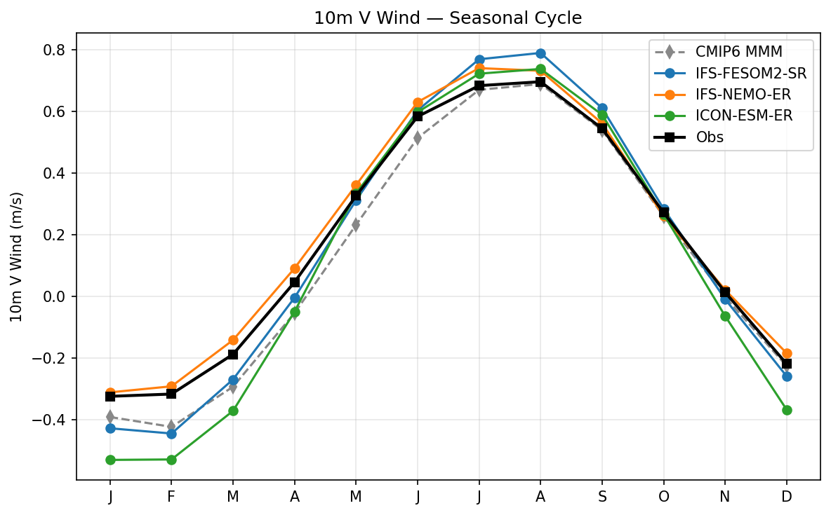
The global mean 10m meridional (V) wind seasonal cycle shows a robust observational pattern of net northward flow in boreal summer and southward flow in boreal winter, which the high-resolution models capture in phase but generally overestimate in amplitude.
Key Findings
- All models reproduce the phase of the ERA5 seasonal cycle, with net northward flow peaking in August and net southward flow peaking in January/February, reflecting the global asymmetry of the Hadley circulation.
- Most high-resolution models exaggerate the amplitude of the seasonal cycle relative to ERA5. For instance, IFS-FESOM2-SR and IFS-NEMO-ER overestimate the August peak by ~0.1 m/s.
- ICON-ESM-ER exhibits a strong negative bias in boreal winter (DJF), reaching global means of ~-0.55 m/s compared to the ERA5 value of ~-0.32 m/s, implying excessively strong southward cross-equatorial flow.
- IFS-NEMO-ER shows excellent agreement with ERA5 during the boreal winter (DJF) minimum but deviates significantly during the boreal summer maximum.
Spatial Patterns
The cycle is characterized by a sinusoidal evolution with a summer maximum (~0.7 m/s in ERA5) and winter minimum (~-0.3 m/s in ERA5). The positive values in JJA correspond to the strong cross-equatorial flow into the Northern Hemisphere (e.g., Somali Jet, Asian Monsoon), while negative values in DJF reflect flow into the Southern Hemisphere.
Model Agreement
While phase agreement is high across all models (including CMIP6), amplitude varies significantly. The high-resolution EERIE models generally show stronger seasonal extremes than the CMIP6 Multi-Model Mean, particularly in summer. IFS-NEMO-ER provides the best match for the winter minimum, while no model perfectly captures the summer peak magnitude without bias.
Physical Interpretation
The global mean V-wind is a residual metric indicating net cross-equatorial mass flux and the asymmetry of the Hadley cells. The positive bias in summer in IFS models suggests an overly strong SH-to-NH surface branch of the Hadley cell or intensified monsoon circulation. The strong negative bias in ICON in winter suggests an overly vigorous NH-to-SH winter circulation. These biases likely stem from errors in meridional SST gradients or ITCZ positioning.
Caveats
- Global mean V-wind is a small residual of large opposing regional flows; small systematic errors in regional circulation (e.g., ITCZ location) can produce large relative errors in the global mean.
- Differences between IFS-NEMO and IFS-FESOM (which share an atmospheric component) suggest that ocean model formulation and resulting SST patterns significantly modulate these global atmospheric circulation residuals.